Integrating AGNOSTOS gene categories into anvi'o projects


Table of Contents
Anyone who studies microbial life through genomes or metagenomes often runs into situations where they find out that a large proportion of their genes do not have any functional annotation. Indeed, as of today 40% to 60% of predicted genes from genomes or metagenomes have no significant homology to genes with known or predicted functions in public databases. Which is only getting worse as we sequence more and more microbiomes from around the globe. To ameliorate the inaccessibility of genes of unknown functions, we, as in Vanni et al. (2021), have recently introduced AGNOSTOS, a computational framework that aims to help microbiologists integrate all genes found in genomes and metagenomes into their ecological and evolutionary investigations. We strongly recommend for anyone who is interested in this topic to also read this blog post by  , where he describes the origins of AGNOSTOS, categories of gene-clusters it produces, and discusses the future of unknown genes in microbiomes.
Our study demonstrated that the AGNOSTOS workflow was able to shed light on the unknown sequence landscape of microbiomes from oceans and the human body by revealing thousands of lineage-specific genes of unknown function and their ecology. But, we were also motivated to turn AGNOSTOS into a resource that empowers researchers to explore genes of unknown functions in their own data sets. Thus, we created this tutorial to demonstrate how to integrate AGNOSTOS gene categories into anvi’o projects using AGNOSTOS-DB.
Even though the tutorial explains the key steps in this integration for anvi’o projects, we are hoping that the example input and output files will enable anyone to be able to implement this workflow independent of tools.
Like many things in our work, the tutorial is a work-in-progress. While we continuously improve it, we would be happy to benefit from your input. Please feel free to reach out to us if you have any questions.
Setting up the stage
The sole purpose of this subsection is to help you download the necessary data to be able to follow the tutorial using the example dataset we have used here. If you want to go straight to data analysis, feel free to skip this section.
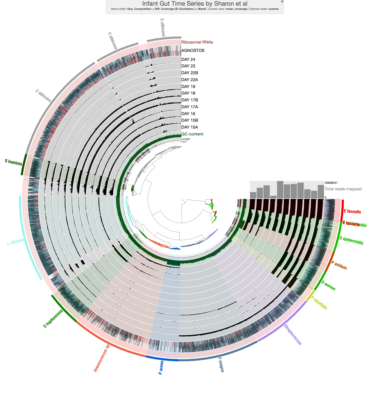
Throughout the tutorial, we will use the Infant Gut Dataset (IGD) as an example project from Sharon et al., 2013. First, however, you should follow these instructions to get the necessary information from an anvi’o project to annotate your genes with AGNOSTOS categories.
To start, please first follow the download instructions in the IGD tutorial here to get the contigs database in your working directory.
$ ls
AUXILIARY-DATA.db  CONTIGS.db  PROFILE.db  additional-files/
If the above is what you see in your work directory, then you are good to follow the rest of the tutorial:
Running AGNOSTOS with data from anvi’o
The purpose of this section is to demonstrate how to extract the necessary data files from an anvi’o project to run the AGNOSTOS workflow on them.
Extracting data from anvi’o
The first step is to export the gene sequences from the contigs database using the anvi’o program anvi-get-sequences-for-gene-calls:
anvi-get-sequences-for-gene-calls -c CONTIGS.db \
                                  --get-aa-sequences \
                                  -o infant_gut_genes.fasta
Next, we need the gene completion information i.e. does a gene contain both a start and stop codon? This can be found in the gene-calls-txt which can be extracted from your contigs database. To do this, we can use the program anvi-export-gene-calls:
anvi-export-gene-calls -c CONTIGS.db \
                       --gene-caller prodigal \
                       -o infant_gut_gene_calls.tsv
And that’s it!
At this point, we have all the necessary files to run the AGNOSTOS-workflow, namely the gene amino acid sequences (infant_gut_genes.fasta) and the gene completion information (infant_gut_gene_calls.tsv).
Running AGNOSTOS
AGNOSTOS gene categories
Before we start, let’s have a refresher on AGNOSTOS gene annotation categories discussed in Antonio’s blog post:
- Known with Pfam annotations (K): genes annotated to contain one or more Pfam entries (domain, family, repeats or motifs) but excluding the domains of unknown function (DUF).
- Known without Pfam annotations (KWP): which contains the genes that have a known function but lack a Pfam annotation. Here we can find intrinsically disordered proteins or small proteins, among others.
- Genomic unknown (GU): genes that have an unknown function (DUF are included here) and found in sequenced or draft genomes
- Environmental unknown (EU): genes of unknown function not detected in sequenced or draft genomes, but only in environmental metagenomes or metagenome-assembled genomes.
The purpose of this section is to demonstrate different ways of utilizing AGNOSTOS depending on the computational resources you have available and the kind of information you want to learn about your unknown sequences. The easiest way to take advantage of AGNOSTOS is to run a profile search of the AGNOSTOS-DB clusters against predicted ORFs from your sequencing data. This will quickly annotate your sequences and tell you about the landscape of your unknown sequencing space. Additionally, you can leverage the metadata associated with each AGNOSTOS cluster annotation, including its lineage specificity, niche breadth, etc.
However, running AGNOSTOS integrates your sequences into the AGNOSTOS-DB clusters or potentially creates new clusters if your genomes and metagenome have novel homologous sequences (go read about that here). The concept of ORF integration is key here because we are not trying to annotate the IGD ORFs. Instead, we are attempting to insert the IGD ORFs into the extant AGNOSTOS clusters that already have metadata associated with them (read more about it here). Thus, integration allows for the entire dataset of ORFs to be used rather than alignment-based methods where one filters for best hits.
The AGNOSTOS-workflow is a complex workflow that relies on many external dependencies. Furthermore, to achieve high sensitivity levels, some of their steps are computationally expensive for large datasets. Currently, AGNOSTOS, although fully functional, should be considered proof of concept of what can be done. At the moment, we are working to make it more accessible and less resource-intensive. This tutorial is the starting point for our plans to integrate an optimized version of AGNOSTOS into anvi’o.
Regardless of which way you decided to use AGNOSTOS we will visualize the data in the next section.
To get started please clone the AGNOSTOS repo:
git clone https://github.com/functional-dark-side/agnostos-wf.git && cd agnostos-wf
Easy mode - quickly annotated sequences with AGNOSTOS categories
Here we will quickly annotate the IGD dataset with AGNOSTOS categories, download the AGNOSTOS-DB profiles and cluster categories.
First, download the AGNOSTOS-DB profiles and cluster categories here:
# Make a home for the AGNOSTOS data
mkdir -p IGD_agnostos

# Download and unzip AGNOSTOS profiles
curl -L https://api.figshare.com/v2/file/download/23066963 -o IGD_agnostos/GC_profiles.tar.gz
tar -zxvf IGD_agnostos/GC_profiles.tar.gz

# Download and unzip AGNOSTOS cluster categories
curl -L https://api.figshare.com/v2/file/download/23067140 -o IGD_agnostos/cluster_ids_categ.tsv.gz
gunzip IGD_agnostos/cluster_ids_categ.tsv.gz
Next, run the profile search.
Please conda install mmseqs2 to run this profile search
Profile_search/profile_search.sh --query infant_gut_genes.fasta \
			         --clu_hmm IGD_agnostos/GC_profiles/clu_hmm_db \
			         --clu_cat IGD_agnostos/cluster_ids_categ.tsv \
			         --threads 10
Hard mode - integrate sequences into AGNOSTOS-DB
Some steps of AGNOSTOS uses MPI compiled programs to be able to process large data sets. It also uses SLURM to distribute many small jobs across many nodes. Although it might work in commodity hardware after having all dependencies installed, we only have tested it in a cloud or HPC infrastructure. Soon we hope to provide Singularity images to make the whole process way more accessible.
Installation instructions for AGNOSTOS can be found here. Once you’ve completed the installation on your HPC come back here and continue the tutorial. If you have any trouble installing AGNOSTOS, don’t hesitate to open an issue here
Download the goods
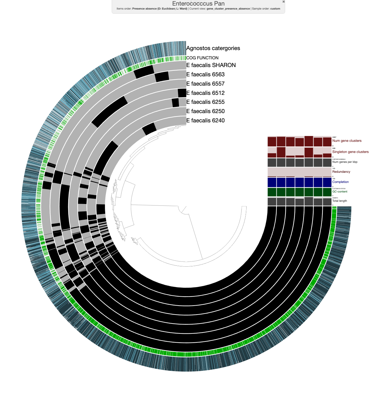
This section will go over how to integrate and visualize AGNOSTOS categories in your anvi’o projects. To have some fun, Chiara Vanni kindly integrated all of the ORFs from the IGD metagenomes using AGNOSTOS. Additionally, she integrated the ORFs from 6 E. faecalis so we can investigate AGNOSTOS categories in the context of a pangenome.
Please download these files to start the analysis:
# Make a home for the AGNOSTOS data
mkdir -p IGD_agnostos

# Download AGNOSTOS integrated IGD metagenomic
curl -L https://api.figshare.com/v2/file/download/28329447 -o IGD_agnostos/IGD_genes_summary_info_exp_coverage.tsv

# Download AGNOSTOS integrated E. faecalis genomes
curl -L https://api.figshare.com/v2/file/download/24028730 -o IGD_agnostos/IGD_ext_genomes_summary_info_exp.tsv
AGNOSTOS produces a very extensive output. here you can find a description of all the fields reported. For this tutorial, we cherrypicked some of them.
Now you are ready to import the AGNOSTOS output for your genes back into your anvi’o project.
What type of results AGNOSTOS provides?
Let’s have a look at what is inside of the file IGD_agnostos/IGD_genes_summary_info_exp_coverage.tsv. If you have installed the awesome csvtk you can easily check the contents with:
csvtk csv2md -t <(head -n4 IGD_agnostos/IGD_genes_summary_info_exp_coverage.tsv)
| cl_name | gene_callers_id | contig | gene_x_contig | cl_size | category | pfam | is.HQ | is.LS | lowest_rank | lowest_level | niche_breadth_sign | is.singleton | ground_coverage |
|---|---|---|---|---|---|---|---|---|---|---|---|---|---|
| 40423550 | 0 | Day17a_QCcontig1 | 1051 | 1 | KWP | NA | FALSE | FALSE | NA | NA | NA | TRUE | NA |
| 32886021 | 1 | Day17a_QCcontig1 | 1051 | 3 | K | Glycos_transf | FALSE | FALSE | NA | NA | NA | FALSE | 0.000257075416579027 |
| 16622933 | 2 | Day17a_QCcontig1 | 1051 | 3606 | K | Glycos_transf_1 | FALSE | FALSE | NA | NA | Broad | FALSE | 0.0153310430250765 |
Some of the interesting columns to check are the cluster size (cl_size); to which category the gene cluster belongs (category); if the gene cluster is high-quality (is.HQ); if it is lineage-specific, and which rank and level (is.LS, lowest_rank, lowest_level); and its environmental distribution based on the metagenomes used to build the seed DB (niche_breadth_sign).
We added an extra column that is not yet integrated into the workflow (ground_coverage) that provides the taxonomic coverage of a gene cluster related to a base taxonomy; the larger the number, the more taxa that have this gene cluster. This metric is one of the outputs of an experimental application of AGNOSTOS to identify contamination in MAGs, where we flag potential contaminants at the contig level (and even within a contig, identifying misassemblies, relevant for ancient metagenomics). The method exploits the information contained in all genes in a MAG, and it considers things like the presence of prophage regions or mobile genetic elements. This is the beauty of gene clusters, where one can combine function and taxonomy. We will write soon another blog post describing the method and how it can help to automatize the manual curation of bins.
Now you are probably wondering, how many KNOWNS and UNKNOWNS do we have? Let’s figure it out with a little of awk-fu (you will need GAWK 4):
$ gawk 'NR>1{a[$6]++;}END { PROCINFO["sorted_in"] = "@val_num_desc"; for(n in a ){printf "%s: %s (%.2f%)\n", n, a[n], 100*(a[n]/(NR-1))}}' IGD_agnostos/IGD_genes_summary_info_exp_coverage.tsv
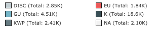
K: 18576 (57.56%)
GU: 4506 (13.96%)
DISC: 2851 (8.83%)
KWP: 2406 (7.45%)
NA: 2095 (6.49%)
EU: 1840 (5.70%)
As expected, the majority of the ORFs (57%) are part of the Known (K) fraction. Then the next category with more ORFs is the Genomic unknowns (GU). The category DISC are those ORFs that have been discarded during the cluster validation step, we are quite conservative here. Then, there is a category with the name NA that contains all ORFs that are most likely gene miscalls. Some of the contigs have many Ns and we also integrated the PRODIGAL predictions for Candida, in both cases, we might have many spurious ORFs. AGNOSTOS will not discard them, but they will end up as singletons. As a side note, for the tutorial we integrated the singletons after being classified and refined.
Import AGNOSTOS into an anvi’o
Whether you have your AGNOSTOS data tables or have downloaded the pre-calculated datasets above, now it’s time to get the AGNOSTOS data back into anvi’o. The first step will be to import the data as functions into the IGD contigs database (check out this post if you have more questions about anvi’o functions tables). This will make it easy to explore the AGNOSTOS categories in the context of assembled contigs and read recruitment results in the anvi’o interactive interface!
Import AGNOSTOS data into the IGD contigs database:
anvi-import-functions -c CONTIGS.db -p AGNOSTOS -i IGD_agnostos/IGD_genes_summary_info_exp_coverage.tsv
Metagenomics applications
Now that we have imported the AGNOSTOS categories into our contigs database, let’s check out the distribution of categories in metagenomic-assembled genomes (MAGs) from the IGD metagenome dataset:
First, let’s import some bins ") made:
made:
anvi-import-collection additional-files/collections/merens.txt \
                       --bins-info additional-files/collections/merens-info.txt \
                       -p PROFILE.db \
                       -c CONTIGS.db \
                       -C default
Since we already imported the AGNOSTOS output into anvi’o, we can immediately visualize the results like this:
anvi-interactive -p PROFILE.db -c CONTIGS.db -F AGNOSTOS
So now we have the data integrated and ready to be used in anvi’o. For example, you can do a global analysis like the one we did with Tom Delmont with the SMAGS or you can use some of the associated metadata to the gene clusters. Below we use the AGNOSTOS metadata for environmental distribution and gene cluster taxonomic coverage to select which ORFs with unknown functions (Genomic unknowns) would be interisting to explore first:

For example, if we are interested in finding potential new marker genes, we can select the Genomic unknowns that have a broad environmental distribution and a large taxonomic coverage. Another direction we can go is to find ORFs with unknown function that might be associated with very specific taxonomic groups and give them a fitness advantage allowing for broad distribution. To find these ORFs, we can select those with a broad environmental distribution but very limited taxonomic coverage. These are just random thoughts for the tutorial, but we hope that you can see the potential of being able to access to the unknown fraction when you are exploring your data.
Pangenomic applications
We are working on this section! Once we are done, this section will include instructions to add a proportion of AGNOSTOS categories for each gene cluster in a given anvi’o pangenome as a layer:
Conclusion
The AGNOSTOS workflow from Vanni et al., 2020 provides a path forward to utilizing all genes from microbiomes and integrates seamlessly into your standard metagenomic or pangenomic workflow as seen above using anvi’o. We hope this brief introduction will catalyze your future microbiomes analyses!
Please refer to our recent preprint Unifying the known and unknown microbial coding sequence space and blog post by Antonio for background and technical details on how to illuminate the genes of unknown function.
“To help you stop having to sweep the unknown under the carpet, we are simply removing the carpet.” -