'Omics Vocabulary
Table of Contents
- All things ‘omics
- Sequencing reads
- Reference sequence
- Read recruitment
- Coverage
- Detection
- Non-specific read recruitment
- Contig
- Metagenomic binning
- Differential coverage
- Tetra-nucleotide frequency
- Metagenome-assembled genome (MAG)
- Single amplified genome (SAG)
- Population
- Community
- Metagenome
- Metatranscriptome
- Virome
- Pangenome
- Metagenomics
- Metatranscriptomics
- Pangenomics
- Phylogenomics
- Gene cluster
- Single-nucleotide variant (SNV)
- Single-copy core gene (SCG)
- Hidden Markov Models (HMMs)
- Completion
- Redundancy
- Microbiota
- Microbiome
- Tree of life
- De novo assembly
- De Bruijn graph
- Metabolite
- Metabolomics
- Metaproteomics
- Strain
- Haplotype
- Orthologous genes
- Paralogous genes
- All things anvi’o
The purpose of this document is to create a resource that defines commonly used terms in microbial ‘omics.
We initially wanted to create a resource just for the terms we commonly use in anvi’o, especially those that are specific to the platform. However, we concluded that including definitions for a larger set of terms (including those that are common in ‘omics studies) would be the only way to have a cohesive document.
Please keep in mind that this is an evolving resource. Please help us improve it.
If you have any questions or concerns, you can always find us on anvi’o 
Contributors
The vocabulary is maintained by  and
and ") , it is here thanks to the contributions of
, it is here thanks to the contributions of  ,
,  , Shiva Thapa,
  , and Valentyn Bezshapkin.
All things ‘omics
This section defines terms that are commonly used in ‘omics studies.
Sequencing reads
Commonly used to define the raw output of a sequencer. These are strings of the alphabet {A, C, T, G}, representing nucleotide sequences of the input DNA or RNA.
Reference sequence
A sequence that you know something about. In the context of metagenomics, it often refers to a sequence that one uses for read recruitment.
Read recruitment
A set of computational strategies to align sequencing reads to one or more reference sequences. Also known as read mapping.
In the context of metagenomics, read recruitment allows one to estimate whether a given sequence is present in a given metagenome. This is done by ‘recruiting’ all reads from a metagenome that matches to any part of the reference sequence. Understanding this strategy, along with its power and caveats, is one of the most important steps to fully appreciate most ‘omics strategies and the ways they lend themselves to study the ecology and evolution of microbial populations.
Read recruitment typically yields two quantities to make sense of a given sequence in the context of a given metagenome: coverage, and detection.
You can find here a simple, introductory hands-on tutorial to read recruitment and profiling. The following video can help beginners appreciate some of the fundamental aspects of read recruitment:
Coverage
Average number of sequencing reads that map to each nucleotide position in a reference.
Also known as “depth of coverage”.
Detection
The proportion of nucleotides in a given reference sequence that are covered by at least one short read.
The detection metric can help determine whether the coverage of a sequence is likely due to non-specific read recruitment:
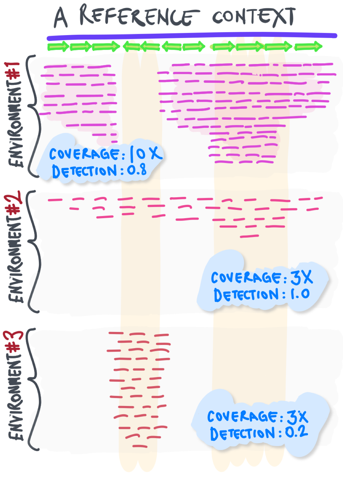
Also known as ‘breadth of coverage’.
Non-specific read recruitment
Recruitment of short reads from an environment to a reference sequence context due to local sequence homology between unrelated populations (i.e., recruiting reads from an environment even if they are not coming from a population of interest). This signal can result in variation in coverage values, or result in misleading conclusions regarding the presence of a population in a given environment due to incorrect coverage estimates. Not coverage, but the detection metric can be useful to identify cases of non-specific read recruitment.
Contig
A contiguous segment of DNA that is often ‘assembled’ from short reads or long rads, but still represents only a fraction of the longer context to which it belongs.
Assembly software often takes short metagenomic reads and yields a list of contigs. Although their lengths vary depending on a myriad of factors, contigs are often orders of magnitude longer than short reads that were assembled, which makes them suitable for downstream efforts that may include gene calling, functional and/or taxonomic annotation, and/or metagenomic binning. Contigs often become reference sequences for read recruitment analyses.
Metagenomic binning
A set of computational strategies that aims to identify and put together contigs that belong to the same population. These strategies often use differential coverage of contigs (when multiple samples are present) and/or sequence composition information (such as tetra-nucleotide frequency).
The following video aims to offer an introduction to concepts in metagenomic binning:
Differential coverage
Change in coverage of a reference sequence across multiple samples. This statistic is one of the essential information for most binning algorithms.
Tetra-nucleotide frequency
The ratio of all 4-nucleotide words in a given contig. The tetra-nucleotide frequency is largely preserved throughout microbial genomes, which enables the identification of distinct contigs that likely originate from the same population.
Learn more about how k-mer frequencies are calculated:
Metagenome-assembled genome (MAG)
A genome that is reconstructed or recovered from a metagenome. MAGs are typically reconstructed from short reads via de novo assembly and metagenomic binning strategies, from long reads, or from a combination of strategies that makes use of both short reads and long reads.
A MAG can be a single contig or a collection of contigs that, in theory, collectively represent a single microbial organism. Although, binning can lead to errors. Quality of a MAG can be assessed by completion and redundancy of single-copy core genes, although, these estimates may not be conclusive. Despite challenges associated with them, MAGs have played essential roles in expanding the tree of life and shedding light on environmental microbiomes and viromes.
Single amplified genome (SAG)
The term single amplified genome is used to refer to a DNA sequenced from an individual cell. The amount of DNA in a cell is extremely low, therefore it should undergo a whole genome amplification (WGA) prior to analysis with modern sequencing methods. Even trace amounts of contaminant DNA influence SAG quality substantially. Thus, the preprocessing step requires an application of specialised instrumentation, such as flow cytometry, microfluidics, and micromanipulators.
Population
Population is an classic ecology term, and thus microbial ecology, that includes all the conspecific individuals from a given ecosystem. In the practice, microbial ecologists often use population to refer to groups of organisms at different taxonomic levels. One of the operational definitions our group often uses suggests that a population is an assemblage of co-existing microbes in an environment whose genomes are similar enough to map to the context of the same reference genome.
Population is often wrongly used instead of community.
Community
The group of all organisms living in a given ecosystem is called community. It is the living portion of an ecosystem. A community can also be defined as the group of all populations in an ecosystem.
Metagenome
The entire DNA content of an environment. Since most environments harbor many different organisms, the metagenome includes genetic information from a large collection of genomes. High-throughput sequencing of metagenomes produce tremendous amount of sequencing reads that can be used for assembly or read recruitment.
On all things ‘meta’
In general, if you see the prefix ‘meta’ in front of an ‘omics term, it means that you are extending that term to apply to all the things within a given sample. For example, the metatranscriptome is the set of transcriptomes from every population in your sample. The metametabolome are all the metabolites coming from all organisms in an environment and so on. In case that’s hard to remember, you can think of the ‘All the Things’ meme.

Works for us. :)
Metatranscriptome
The entire RNA content of a given environment. Unlike metagenomes, metatranscriptomes can shed light on the activity of environmental populations. But they bring unique challenges, such as the short half-life of RNA molecules, and secondary-structure driven variation in their coverages.
Virome
A metagenome derived from the viral fraction of a sample. OR, the assemblage of viruses in a specific sample or environment. Yes, the same word ended up designating two different concepts, sorry about that… Unfortunately, at this point, there are no great alternative for either use of “virome”, so both are regularly found in the literature and the specific meaning typically has to be deduced from context (fortunately, this is often relatively straightforward).
In the first case, “Virome” is used as shorthand for “Viral metagenome”. Pragmatically, a virome is a metagenome generated from a sample that has been specifically processed to be (i) enriched in viral particles and/or (ii) depleted in cellular (micro)organisms, through a combination of filtering, precipitation, and other (almost) magic tricks. These datasets are sometimes designated as “metavirome”, but this terminology is also not satisfying because it does not follow the use of “meta” as a prefix to “extend that term to all the things within a given sample” (see Metagenome above). Here instead, the notion of “extend to all the things” is already built into “virome”, and the meta prefix is redundant.
In the second use, “Virome” is essentially the counterpart of “Microbiome”, and is built the same way: while the microbi-ome would designate the community of microorganisms found in a single habitat, the vir-ome would designate the community of viruses found in this habitat. This makes a lot of sense, and is typically the definition provided by encyclopedia. The only (major) flaw of course is that this term was already used to designate “viral metagenomes”.. Sadly, the fact that (viral) metagenomics is often the method of choice to explore “viromes” only adds to the confusion.
Pangenome
From a computational standpoint, the term pangenome broadly refers to the entire collection of genes found in two or more genomes. See pangenomics for more.
Metagenomics
The study of environmental metagenomes.
Metatranscriptomics
The study of environmental metatranscriptomes.
Pangenomics
The family of computational strategies that determine the pangenome and make it accessible as a framework to study relationships between a set of genomes through gene clusters.
The following video aims to offer an introduction to concepts in pangenomics:
Phylogenomics
The practice of inferring evolutionary history and relationships between different organisms, based on genomic differences across multiple conserved genes.
The following offers an introduction to basic concepts of this approach that yields phylogenomic trees:
Gene cluster
Fundamental units of pangenomes which appear in the literature also as ‘protein clusters’, ‘orthogroups’, ‘groups of orthologous genes’, or ‘operational protein families’ (and they should not be confused with biosynthetic gene clusters which describe functionally related genes that belong to the same operon in a single chromosome).
Commonly used computational strategies for pangenomics that consider entire contents of input genomes determine gene clusters typically by (1) identifying all genes among a set of genomes, (2) computing similarities between each gene using translated DNA sequences, and (3) determining which genes are homologous enough to be described in the same cluster. Hence, a gene cluster in a given pangenome corresponds to a de novo identified virtual construct that contain one or more genes from one or more genomes.
For a tutorial on how to do pangenomics with anvi’o, see this page.
On all things ‘pan’
Where ‘meta’ indicates that we apply our analysis across all populations in a given sample, ‘pan’ indicates that we apply our analysis within a single group. We couldn’t find a good meme for ‘pan’, so please accept this analogy instead: Imagine you have a frying pan, in which you are making an omelet. To get the nutritional information for that omelet, you analyze what is in the pan. Some ingredients will contain the same nutrients, like protein or carbohydrates. Other nutrients, like specific vitamins, will be exclusive to certain ingredients. So the ‘pan’-nutrients will include all the nutrients within the frying pan, regardless of which ingredient they came from (see what we did there?).
Single-nucleotide variant (SNV)
A nucleotide position where the identity of all bases mapping to this position varies (beyond the expected rate of sequencing error).
SNVs are characterized by (1) the position in the reference sequence where the difference occurs, and (2) a frequency vector that quantifies the frequency of nucleotide identities that mapped onto that position. See this page for a lengthier discussion of SNVs. Also see the definition of single-codon variant and single-amino acid variant.
Single-copy core gene (SCG)
A gene that is found in the vast majority of genomes and yet occurs only once within a single genome.
Single-copy core genes play a central role in phylogeneitcs, phylogenomics, as well as estimating genome completion and redundancy.
Commonly used SCGs can be identified across a set of genomes through sequence homology searches (via hidden Markov models, BLAST, or other means). For relatively closely related genomes, SCGs can also be identified de novo through pangenomics.
The number of SCGs will decrease with decreasing resolutions of taxonomy. For instance, the number of SCGs across a set of genomes that belong to the same phylum will typically be much smaller than the number of SCGs across a set of genomes that belong to a same genus within that phylum, and so on. At the domain level there exists a small set of ribosomal proteins that are both core and single-copy across a very large number of genomes that span eukarya, archaea, and bacteria and lead to comprehensive analyses of the tree of life through phylogenomics.
Hidden Markov Models (HMMs)
A Markov model allows us to predict/describe a future state, given the knowledge of current state (observation) in the sequence. The past state is not important in predicting the future outcome. To summarize, the system state at a given time point “t+1” is dependent upon the state at time point “t”. Hidden Markov Models are the Markov models where the states are hidden or not directly unobservable.
HMMs have been widely used in bioinformatics for various forms of sequence analysis, including database searches, gene prediction, and solving pairwise and multiple sequence alignment problems. Many problems in biological sequence analysis require associating new DNA or amino acid sequences with known protein families or phylogenetic branches through ‘sequence-based homology detection’.
HMMs have certain advantages at solving the problem of homology detection. For instance, in comparison to BLAST, (1) HMMs exhibit higher sensitivity to identify remote homologs, (2) can assign position-specific gap penalties, which leads to better depiction of changes occurring at a conserved vs variable region, and (3) can compute a consensus alignment considering all possible alignments, rather than a singular best-scoring alignment, which yields increased efficiency in predicting true homologs.
Completion
A rough estimate of how completely a set of contigs represents a full genome based on the presence or absence of single-copy core genes (SCGs) they contain. So theoretically, the higher the percentage of SCGs found in a genome, the more complete the genome. Of course, popular SCGs are determined through the analyses of isolate genomes that are available, thus, the accuracy of their predictions may be limited when this approach is applied to genome bins that represent populations from poorly studies clades of life. Even for genomes of well-studied organisms, our methods to identify these genes in genomes may prevent us from getting to 100% completeness.
Redundancy
A measure of how many copies of each single-copy core gene (SCG) is found within a genome. Due to the special single-copy nature of SCGs, their occurrence as multi-copy in a genome is commonly used as an estimate of the level of ‘contamination’ within a genome bin (i.e., higher values of redundancy may indicate that more than one population may be contributing to a given genome bin). However, interpretations of ‘contamination’ as a function of redundancy may not be straightforward as some genomes may have multiple copies of genes that are in general single-copy, thus drawing conclusions regarding contamination from redundancy data may not be appropriate. That said, the lack of redundancy in a genome does not necessarily mean the lack of contamination, either. Since contaminant contigs that do not include SCGs will not be in the radar of these estimates. Such contamination can especially affect metagenome-assembled genomes, and lead to the formation of misleading branches in phylogenomics and excessive number of singletons in pangenomics analyses.
Microbiota
In macroecology, the biota is the group of flora and fauna inhabiting the same place. Similarly, the microbiota applies to microorganisms. The term microbiome is often erroneously used instead.
A relevant commentary by Berg et al: Microbiome definition re-visited: old concepts and new challenges.
Microbiome
A biome is an biological subdivision that reflects the biota and its environment. A biome is constrained by the physico-chemical characteristics and biota that defines it. In macroecology, the biomes are often defined in part based on the climatic conditions, e.g. tundra biome, desert biome… In another way, a biome is the combination of the biota and the characteristics of its environment. A microbiome would be defined in a similar way at a much smaller scale. Due to the variability of the physico-chemical characteristics and the biota at very small distances, a microbiome can occuppy extremely small extensions in opposition at the large scale of traditional biomes.
The term microbiome is often misused. For example, microbiome analysis services only really analyse the microbiota (normally only stool microbiota), as they don’t collect physico-chemical parameters from the samples.
Tree of life
A tree of life (ToL) is a conceptual research tool, which allows for the exploration of relationships between organisms. Evolution is a slow process, that changes organisms bit by bit. Therefore, by quantifying similarities of genetic code it is possible to hypothesise which organisms are closely related from an evolutionary standpoint. It is important to note that not a given ToL does not necessarily represent the true evolutionary history of organisms it includes, as the underlying data that leads to such inferences are typically noisy, events that may have occurred in the past (i.e., horizontal gene transfer) are not always available to models, and different sets of genes may yield different interpretations of the ancestral relationships between the same set of organisms. Also see phylogenomics.
De novo assembly
Modern high-throghput sequencing technologies such as Illumina cannot read the entirety of chromosomes, and instead produce short fragments. The process of assembly aims to extend short reads into longer contiguous segments of DNA or RNA (i.e., contigs) to reconstruct the original sequence. Historically, assembly process relied upon known genomes that were present in databases. In contrast, the de novo approach allows assembly without prior knowledge of the original sequences. The algorithms used for this task are varied, but the most popular tools for short-read assembly rely on de Bruijn graphs.
De Bruijn graph
De Bruijn graph is a directed graph, that represents overlaps between sequences through k-mers. Modern assemblers work with k-mers of a particular length or a combination of lenghts through iterative steps. Here is a video by Rob Edwards in which he explains the basic principles of this strategy using a simple example:
Metabolite
Metabolite is a product of the chain of life-sustaining chemical reactions in living organisms. It is usually used for small molecules. They have various functions, such as fuel, structure, signaling, defense, etc. I.e., the main energetic metabolite is adenosine 5’-triphosphate (ATP), which participates in various chemical reactions vital for life.
Metabolomics
The study of metabolites in bulk is called “metabolomics”. It allows for identification of the unique chemical fingerprint of a tissue, organ or organism. In the current state it faces a lot of methodological challenges. Contrary to genomics or proteomics, molecules have distinct physical properties. Thus, the full picture of the metabolic profile is obtained from combination of different methods.
Metaproteomics
Metaproteomics is an umbrella term for experimental approaches that are used for studying proteins in microbial communities. The term was coiled in a similar fashion as “metagenomics” (see above). It involves non-targeted shotgun mass spectrometry. Therefore, it concentrates on post-trascriptionally regulated and transcribed proteins. It is often used complementary to metagenomics.
Strain
Strain is a genetic variant or subtype of a species. It gets tricky if you ask how a species is defined, as there is no single definition. But in order to retain brevity we will stick to the proposed definition, undertanding it as a “fine-grained” resolution of species.
Haplotype
Haplotypes are variant copies of a genome in a population. Contrained to microbiome, it’s two bacterial species that differ by a one or more bases - single nucleotide variants (SNVs).
In modern metagenomics, haplotype recovery is a challenge, because assembly methods rely on consensus of the true haplotypes within a sample. It is additionally complicated with an error rate of sequencing methods (around 1 in 100 bases). In such circumstances low-frequency haplotypes are virtually indistunguishable from noise. Even high-quality, single-molecule, long-read sequencing platforms fail to achieve good accuracy on the single read level.
Orthologous genes
Orthologous genes (or orthologs) are genes present within different organisms, but derived from a common acncestor. I.e. 89-90% of the genes of rat (Ratus Norvegicus) possess a single ortholog in human genome.
Paralogous genes
Paralogous genes (or paralogs) are genes that emerged in result of gene duplication event. They are often present within single species and encode proteins with similar function. I.e. human alpha and beta globulin genes are considered to be paralogous. Paralogs constitute 2/3 of human genome.
All things anvi’o
This section defines terms that are largely specific to anvi’o.
Interactive interface
Highly customizable visualization environment in anvi’o to interact with data. It is integrated into most of the core functionalities of anvi’o, but can also be used with tabular data inputs. See this document for more details.
Split
A fragment of a contig in your anvi’o analysis. Anvi’o, by default, breaks up long contigs you provide into multiple parts, called ‘splits’, purely for visualization purposes so the researcher can distinguish a very long contig from shorter ones. This way, a single contig that represents 1,000,000 base pairs would not have less visual significance than 10 contigs each of which are about 10,000 base pairs. The default split size is 20,000 bp, but you can change this using the --split-length parameter when you generate an anvi’o contigs-db.
Layer
Every concentric circle in anvi’o interactive interfaces (in radial display mode). Visualization of a minimal metagenome in anvi’o interactive interface layers will include the parent, GC-content, and metagenomic samples.
Item
Data points shown in layers. Items can be a lot of things in anvi’o: they will be splits in metagenomic mode, genes in gene mode, gene clusters in pangenome mode, or genome bins in collections mode.
Parent layer
The special layer in anvi’o interactive interfaces that describe which splits belong to which contigs (if your contigs were long enough to be split).
Items organization
The center piece of an anvi’o interactive display that organizes items. It could be a hierarchical clustering dendrogram based on an anvi’o clustering configuration, or a user-provided phylogenetic tree. These organizations can also utilize alphabetical orders, or additional user-provided layers.
Clustering configuration
An advanced description of how you want anvi’o to cluster your contigs. A clustering configuration is described in a text file which specifies things like which data sources you want to use for clustering and how to normalize each data source.
View
Statistic behind the data points shown for a given item in a given anvi’o display. A particular view considers some statistic associated with your items that anvi’o calculated automatically, or provided externally, to produce an informative (and hopefully beautiful) graph. For more information about the types of views in anvi’o, please take a look at this post by Mike Lee.
Contigs database
A self-contained database containing a lot of information associated with your contig (or scaffold) sequences. This includes data that isn’t dependent on which sample the contigs came from, like positions of open reading frames, k-mer frequencies, split start/end points, functional and taxonomic annotations among others. You can initialize a basic contigs database from a FASTA file with the command anvi-gen-contigs-database and supplement it with additional information later in your analysis. See more here: contigs-db.
Profile database
A database containing sample-specific information about your contigs; for instance, coverage information from mapping reads to the contigs in a sample. Single profiles, each of which contains data for a particular sample, can be combined into a merged profile if they link to the same contigs database. The information across samples in a merged profile can be visualized as a ‘view’ in the anvi’o interactive database. See more here: profile-db.
HMM profile
Information about known genes that can be used to search for the presence of these genes (dubbed ‘hits’) in contigs, using Hidden Markov Models. More formally, these profiles probabilistically describe variable and conserved regions in a set of homologous sequences. Anvi’o ships with four HMM profiles of bacterial single-copy core genes, but you can also use your own custom HMM profile if you so desire.
Variability profile
Information on residue variants across samples. These variants, whether they are SNVs, SCVs, or SAAVs, are usually identified for each sample when a profile database is generated for the sample. This information can later be combined across samples into a variability profile using the command anvi-gen-variability-profile. For an extensive tutorial on how to analyze variability profiles using anvio pleafixed some spelling se refer to this resource.
External gene calls file
A text file containing gene predictions that you obtained from external software, but wish to import into anvi’o when generating your contigs database. This file must follow the format specified here.
External functions file
A text file containing functional predictions that you obtained from external software, but wish to import into anvi’o using anvi-import-functions. This file must follow the format specified here.
External taxonomy file
A text file containing taxonomy information for your genes that you obtained from external software, but wish to import into anvi’o using anvi-import-taxonomy-for-genes. This file must follow the format specified here.
Collection
A virtual construct to store bins of items in an anvi’o profile database. Each collection contains one or more bins, and each bin contains one or more items. These items can be gene clusters, contigs, or other things depending on the display mode. See collection for more information.
Single-codon variant (SCV)
The lazy definition - an SCV is just like a SNV, but for a codon position. The complete definition - A codon position where the entire, 3-base codon identity (there are 64 possible codons) is different between a reference coding region and mapped reads. SCVs are characterized by 1) the position in the reference sequence and 2) the frequency of codons in that position. If you want an even longer explanation, see this page.
Single-amino acid variant (SAAV)
Differences between mapped reads at the amino acid residue level. See this page for a more comprehensive description.
Are you not happy with something? Do you think something is missing? GOOD! Please visit this page and join us in the dark side.