Targeted binning of a novel nitrogen-fixing population from the Arctic Ocean

Table of Contents
- Setting up our story
- A bit of background
- The nitrogen fixation pathway - KEGG vs reality
- Nitrogen fixation in the polar oceans, and an awesome polar ocean dataset
- Estimating metabolism in Arctic Ocean metagenomes
- Looking for evidence of a nitrogen-fixing population
- Determining population identity
- BLAST results for sample N06
- BLAST results for sample N07
- BLAST results for sample N22
- BLAST results for sample N25
- Aligning N06_c_000000000415 and N25_c_000000000104
- Three samples with the same population
- Comparison of nifH genes
- Identifying the associated Cao et al. MAG
- Distribution of Genome_122 in the global oceans
- Targeted binning of the nitrogen-fixing population
- Estimating metabolism for our new MAG
- Final Words
In this blog post, I will demonstrate how to use anvi-estimate-metabolism to find and bin a novel, nitrogen-fixing population from a set of publicly-available Arctic Ocean metagenomes. Of course, nitrogen fixation is just an example here, and the same technique can be applied to survey metagenomic datasets for microbial populations with other characteristic metabolic capabilities. So if you are interested in learning about how to leverage anvi’o’s metabolism estimation capabilities to go fishing through your data, or if you just can’t get enough of cool marine nitrogen fixation stories, keep on reading!
This post also doubles as a reproducible workflow. Feel free to download the associated datapack from this link (or use the bash commands below) and follow along with the commands - or, go your own way and explore the data yourself. The commands below were written for anvi’o v7.1. If you have a newer version of anvi’o and find a command that is not working - sorry. We don’t always retroactively update these posts as anvi’o evolves. Please let us know and we’ll see if we can help.
# Download tutorial datapack (the unzipped datapack is 3.4 GB in size)
curl -L -o NIF_MAG_DATAPACK.tar.gz https://api.figshare.com/v2/file/download/31119277

# unzip and cd into working directory
tar -xvf NIF_MAG_DATAPACK.tar.gz && cd NIF_MAG_DATAPACK
Setting up our story
Exciting things are happening right now in the world of marine microbiology. Our friend and colleague Tom Delmont is publishing a cool story about heterotrophic bacterial diazotrophs, or HBDs.
Tom’s paper is now published at The ISME Journal! You can find it at this link. Yay :)
For anyone who doesn’t know, a diazotroph is a microbe that fixes nitrogen. Nitrogen fixation is a very important process that supports all forms of life on Earth by yanking nitrogen atoms from one of the most recalcitrant molecules on earth, N2 gas, and putting them into biologically-usable molecules such as ammonia. It happens quite a lot in the global oceans, so to marine microbiologists, nitrogen-fixing microbes - that is, marine diazotrophs - are a Big Deal.
Marine diazotrophs come in many forms, but not all of them have been getting equal amounts of attention. For instance, cyanobacterial diazotrophs have long been thought to be the most abundant type of nitrogen-fixing microbes in the ocean, and therefore have been the focus of most research related to the subject. Though the existence of non-cyanobacterial, heterotrophic diazotrophs has long been known, their presence was measured through amplicon surveys that targeted a single gene in the nitrogen fixation operon: nifH. These amplicon surveys were also the only way to discuss the relative abundance of heterotrophic diazotrophs in oceans compared to their cyanobacterial counterparts. But there were no actual microbial genomes, which prevented our ability to study their ecology without primer sequences and PCR amplification biases.
A relatively recent study, which took years in the making and shaped large parts of anvi’o, changed this by giving access to the first-ever genomes of heterotrophic diazotrophs. It showed that they were much more abundant than what we could survey with nifH primers and came from taxa that were not previously considered in the context of nitrogen fixation (such as Planctomycetes). The saga of discovering new heterotrophic diazotrophs continues with this new paper by Tom Delmont et al., in which Tom manually curates almost 2,000 metagenome-assembled genomes (MAGs) from co-assemblies of almost 800 ocean metagenomes, and then mines this MAG set for nitrogen fixation genes to find an additional 48 diazotrophs.
The benefits of characterizing all genomes found in ocean metagenomes are obvious. Yet, it is not as obvious how one would survey these metagenomes for targeted genome-resolved insights - for instance, to recover particular genomes that encode metabolic modules of interest, such as nitrogen fixation.
One might suggest that we could automatically bin all genomes from metagenomes, and then survey the nifH genes in them to find diazotrophs (as nifH is the standard marker for nitrogen fixation). But it may not be that simple. Not only there are many things that can go wrong with automatic binning, but perhaps more critically, the presence of a key function from a metabolic module does not necessarily indicate the presence of the metabolic capacity. For instance, the nifH gene can occur in a variety of different contexts, so it is actually necessary to find 6 different nif genes to be sure of a microbe’s nitrogen-fixing capabilities (Dos Santos 2012). As a clear example, when I survey a metagenome from the Southern Ocean, an environment where no microbes that fix nitrogen has ever been found, I find 12 COG annotations of nifH genes. In the case of nifH, one can look for other genes nearby in the same contig, such as nifK, nifD, etc. But what if you are targeting a more complex metabolic capability for which the required genes are more diverse?
This is precisely what anvi-estimate-metabolism enables you to do. Without having to implement a lot of ad hoc steps, you can identify contigs in your metagenomes - prior to binning - that may belong to a specific population of interest that encodes a desired metabolic capacity. anvi-estimate-metabolism is a program that predicts the metabolic capabilities of microbes from genomic or metagenomic data. It combines functional annotations from the KOfam database with KEGG definitions of metabolic pathways to estimate completeness of these pathways and produce easily-parsable output. If you are interested in finding a microbe that has a particular metabolic capability, it is much easier to find it using this output rather than parsing through annotations for individual genes.
And that is exactly how we are going to do it today. As I mentioned at the beginning of this post, we’ll be using anvi-estimate-metabolism to look for a previously-uncharacterized marine diazotroph in a set of Arctic Ocean metagenomes.
A bit of background
Before we get started, let’s talk a bit more about nitrogen fixation. I am by no means an expert in this (or in any particular metabolism, really), so here is a very light summary of the background. Experts, feel free to roll your eyes at me and skip to the good stuff.
Nitrogen fixation is the process of converting gaseous nitrogen (N2) into the more biologically-usable form ammonia (NH3). The resulting ammonia can then be further converted into other bioavailable compounds like nitrate and nitrite. Since nitrogen is an essential component of many biological molecules (amino acids, anyone?), nitrogen fixation is a fairly important process that supports life, in general. Only some ocean microbes, called marine diazotrophs, have the genes that allow them to fix nitrogen, which are (usually) encoded in the nif operon. (Sohm 2011)
The nitrogen fixation pathway - KEGG vs reality
The KEGG module for nitrogen fixation is M00175, and it looks like this (image has been modified with labels):
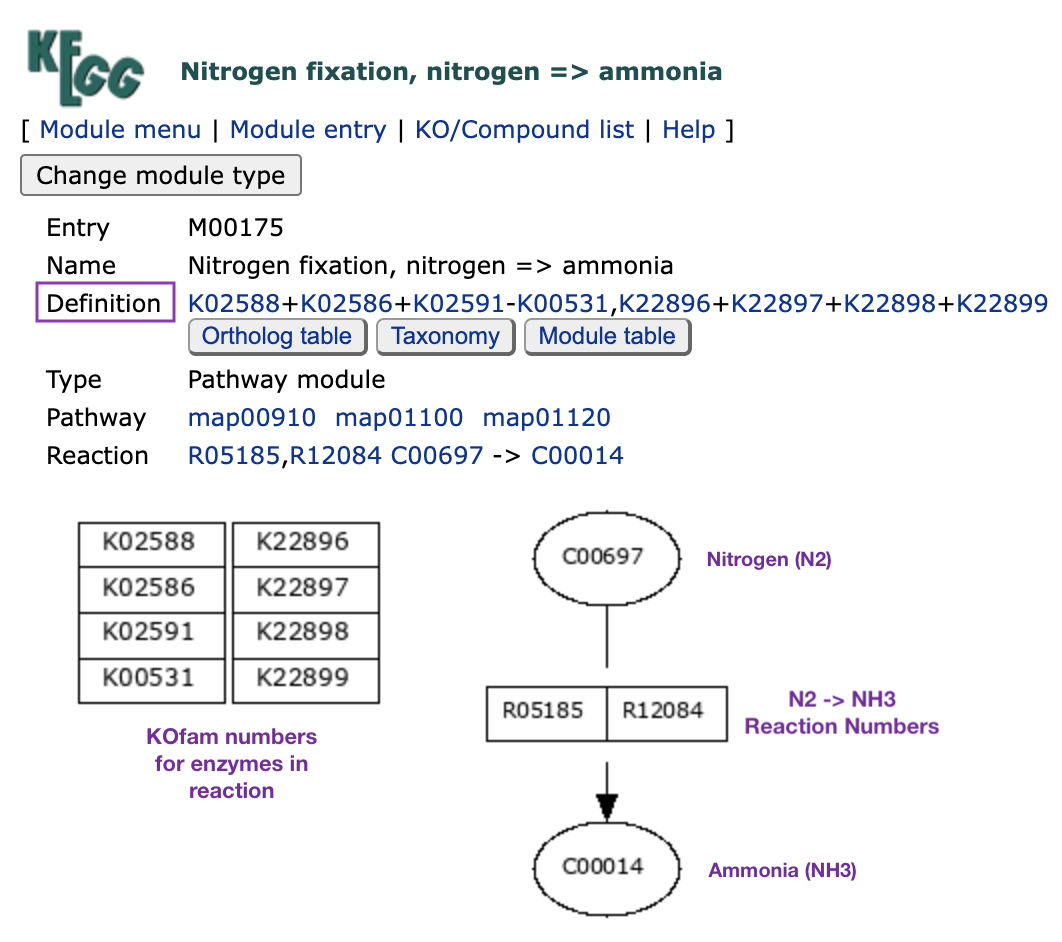
The part of the module that you’ll want to focus on here is the “Definition” line containing the KO numbers for each enzyme required in the pathway (these KOs are also arranged in the rectangular boxes in the bottom-left). You need a nitrogenase enzyme complex to convert nitrogen gas to ammonia, and there are currently only two major versions of this complex: the “molybdenum-dependent nitrogenase” protein complex encoded by genes nifH (K02588), nifD (K02586), and nifK (K02591) of the nif operon; or the “vanadium-dependent nitrogenase” protein complex encoded by genes vnfD (K22896), vnfK (K22897), vnfG (K22898), and vnfH (K22899), of the (you guessed it) vnf operon. The latter complex has been isolated from soil bacteria and is known to be an alternative nitrogenase that is expressed when molybdenum is not available (Lee 2009, Bishop 1980). We’re just going to ignore it, because I have yet to see it in any ocean samples.
You might have noticed that I left K00531 out of the above discussion. That is because this KO is not part of the nif operon - rather, it is the gene anfG, which is part of the alternative nitrogen fixation operon anf. anf encodes an alternate nitrogenase enzyme made up of the components anfHDKG, but anfHDK are very similar to the nifHDK components (Joerger 2021). My best guess as to why anfHDK don’t have their own KOfam profiles is that the nifHDK KOfams can match to these genes. But since anfG is an additional component that is not required for the nif operon, it has its own KO and is labeled as non-essential to the enzyme complex in this module (that is what the minus sign in front of K00531 in the module definition means). This is a very long-winded way of saying that we don’t have to worry about looking for K00531 in our data.
So that means we effectively care about only nifHDK in this module. But wait. While nifHDK represent the catalytic components of the nitrogenase enzyme, it turns out that there are a few other genes required to produce an essential FeMo-cofactor and incorporate it into this complex. At minimum, the extra genes required are nifE (K02587), nifN(K02592), and nifB (K02585) (Dos Santos 2012).
Just so you have a picture of what this should look like, here is a diagram of the nif operon in the Azotobacter vinelandii genome sequence, from Dos Santos 2012:
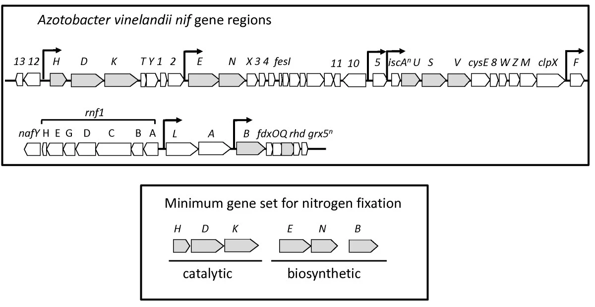
The catalytic genes - those from module M00175 - are located next to each other on the bacterial chromosome. The other required biosynthetic genes are located farther along, with nifE and nifN expressed under the same promoter and nifB isolated from the rest of the genes and expressed under its own promoter.
What this means is that we need to find six genes - preferably located on the same contig - within a metagenome assembly in order to be confident that the metagenome includes a nitrogen-fixing population. We expect to see the same structure as in the diagram above reflected in our metagenome assemblies, meaning that gene groups nifHDK and nifEN are the most likely to end up on the same contig. If you keep reading, you will see that this is indeed the case!
Nitrogen fixation in the polar oceans, and an awesome polar ocean dataset
One aspect of this analysis that makes it a bit more interesting is that we will be working with polar ocean metagenomes. The polar oceans - which are the Arctic Ocean and the Southern Ocean around Antartica - are not typically associated with nitrogen fixation. The vast majority of nitrogen-fixing microbes have been found in non-polar oceans, perhaps because the diazotrophic cyanobacteria that are typically studied tend to be found in warmer waters (Stal 2009), or perhaps because the polar oceans are just not as well-studied as the other oceans. Regardless, in recent times, there have been several reports of nitrogen fixation happening in the Arctic and Antarctic Oceans (Harding 2018, Shiozaki 2020, von Friesen and Riemann 2020). So it is certainly not an unusual or fruitless choice to be searching for nitrogen-fixing microbes in the colder waters of our planet.
We will be using a recently published dataset of Arctic and Antarctic ocean metagenomes by Cao et al. These brave scientists faced the cold to bring the marine science community 60 new samples from 28 different locations in the polar oceans. Their comparative analyses demonstrated that polar ocean microbial communities are distinct from non-polar ones, both in terms of their taxonomic diversity and their gene content. They also reconstructed 214 metagenome-assembled genomes, 32 of which were enriched in the polar oceans according to read recruitment analyses. In their paper, the authors analyzed some metabolic pathways in these MAGs, but notably did not check for nitrogen fixation - maybe because they didn’t expect to find it. But as you will see, it is there to be found.
So without further ado, let’s go through this analysis together :)
Estimating metabolism in Arctic Ocean metagenomes
To start, we need metagenome assemblies of the Arctic Ocean samples from Cao et al.’s dataset. I am fortunate to be colleagues with Matt Schechter, an awesome microbiologist who knows way more about oceans than I do, and who also happened to be interested in this dataset. He downloaded the samples and made single assemblies of them using the software IDBA-UD as part of the anvi’o metagenomic workflow. We are all benefiting from his hard work today - thanks, Matt!
We won’t look at all 60 samples from the Cao et al. paper, only 16 of their surface Arctic Ocean samples (taken from a depth of 0 m).
You do not need the metagenome assemblies to follow the rest of this blog post, but if you would like to have access to the 16 assemblies I am talking about, you can download their contigs databases from this link. But be warned - they will take up 6.5 GB of space on your computer.
When we downloaded these samples, we assigned different (shorter) names to them, so the sample names I will discuss below are different from the ones in the Cao et al. paper. If you want to know the correspondence between our sample names and those in the paper, check out the cao_sample_metadata.txt file in the datapack. You will find their sample names in the sample_name_cao_et_al column.
The first thing that I did with those 16 assemblies was run anvi-estimate-metabolism in metagenome mode. I will show you the commands that I used to do this, but I won’t ask you to do it yourself, because it takes quite a long time (and currently requires an obscene amount of memory, for which I deeply apologize). I created a metagenomes file called metagenomes.txt which contains the names and contigs database paths of each sample, and I wrote a bash loop to estimate metabolism individually on each sample:
while read name path; \
do \
    anvi-estimate-metabolism -c $path \
    --metagenome-mode \
    -O $name \
    --kegg-output-modes modules,kofam_hits; \
done < <(tail -n+2 metagenomes.txt)
If you are determined to run this loop yourself, it is probably only possible on a high-performance computing cluster, in which case you will almost certainly have to give each anvi-estimate-metabolism job more memory than is allocated by default on your system.
What this loop does is read each line of the metagenomes.txt file, except for the first one (the tail -n+2 command skips the first line). Each non-header line in the file contains the name of the metagenome sample (which gets placed into the $name variable) and the path to its contigs database (which gets placed into the $path variable). Therefore, anvi-estimate-metabolism gets run on each contigs database in metagenome mode, and the resulting output files (two per sample) are prefixed with the sample name.
It is possible to run anvi-estimate-metabolism on more than one contigs database at a time, using multi-mode, which you can read about on the anvi-estimate-metabolism help page. However, I did not do this here because I wanted the output for each sample to be printed to a separate output file, for purely organizational purposes.
You will find the resulting output files in the datapack, which you should have downloaded at the beginning of this post. Notice that there are 32 text files, two for each metagenome assembly, in the METABOLISM_ESTIMATION_TXT folder. Let’s take a look at the first few lines of the modules file for sample N02:
cd METABOLISM_ESTIMATION_TXT/
head -n 4 N02_modules.txt
You should see something like this:
| unique_id | contig_name | kegg_module | module_name | module_class | module_category | module_subcategory | module_definition | module_completeness | module_is_complete | kofam_hits_in_module | gene_caller_ids_in_module | warnings |
|---|---|---|---|---|---|---|---|---|---|---|---|---|
| 0 | c_000000008738 | M00546 | Purine degradation, xanthine => urea | Pathway modules | Nucleotide metabolism | Purine metabolism | “(K00106,K00087+K13479+K13480,K13481+K13482,K11177+K11178+K13483) (K00365,K16838,K16839,K22879) (K13484,K07127 (K13485,K16838,K16840)) (K01466,K16842) K01477” | 0.5 | False | K13485,K16842,K07127 | 121398,121397,121396 | None |
| 1 | c_000000000052 | M00001 | Glycolysis (Embden-Meyerhof pathway), glucose => pyruvate | Pathway modules | Carbohydrate metabolism | Central carbohydrate metabolism | “(K00844,K12407,K00845,K00886,K08074,K00918) (K01810,K06859,K13810,K15916) (K00850,K16370,K21071,K00918) (K01623,K01624,K11645,K16305,K16306) K01803 ((K00134,K00150) K00927,K11389) (K01834,K15633,K15634,K15635) K01689 (K00873,K12406)” | 0.4 | False | K00134,K00873,K01624,K00927 | 8515,8519,8523,8454 | None |
| 2 | c_000000000052 | M00002 | Glycolysis, core module involving three-carbon compounds | Pathway modules | Carbohydrate metabolism | Central carbohydrate metabolism | “K01803 ((K00134,K00150) K00927,K11389) (K01834,K15633,K15634,K15635) K01689 (K00873,K12406)” | 0.5 | False | K00134,K00873,K00927 | 8515,8519,8454 | None |
This is a modules mode output file from anvi-estimate-metabolism (which is the default output type). Since we ran the program in metagenome mode, each row of the file describes the completeness of a metabolic module within one contig of the metagenome. What this means is that every KOfam hit belonging to this pathway (listed in the kofam_hits_in_module column) was present on the same contig in the metagenome assembly. This is important, because metagenomes contain the DNA sequences of multiple organisms, so the only time that we can be sure two genes go together within the same population genome is when they are assembled together onto the same contig sequence.
If right now you are thinking, “But wait… if we only focus on the genes within the same contig, many metabolic pathways will have completeness scores that are too low,” then you are exactly correct. It is likely that most metabolic pathways from the same genome will be split across multiple contigs, and their components will therefore end up in different lines of this file. In the example above, contig c_000000008738 contains 50% of the KOs required for the purine degradation module M00546, but perhaps the other KOs in the pathway (such as K01477) also belong to whatever microbial population this is, just on a different contig. Putting many contigs together to match up the different parts of the pathway, while making sure that you are not producing a chimeric population, is a task that requires careful binning.
Luckily for us, the nitrogen fixation module from KEGG (as described earlier in the post) has a couple of helpful characteristics. First, it contains only the 3 catalytic genes, and second, it is encoded in an operon, so those genes are located close together in any given genome sequence. These two things make it much more likely that the entire module will end up within a single contig in our metagenome assemblies, which means it will be relatively easier to find a complete nitrogen fixation module in our metabolism estimation output files.
Looking for evidence of a nitrogen-fixing population
Though M00175 only contains the catalytic portion of our required nif gene set, it is a good starting point for our search. If we look for this module in our metabolism estimation results, we can find out which contig(s) it is located on and use that to guide our search for the remaining genes.
Using modules mode output to find M00175
You can use the following bash code to search for lines describing M00175 in all metabolism estimation modules mode outputs. The code filters the output so that it contains only those lines which have a score of 1.0 in the module_completeness column, meaning that all 3 nifHDK genes are located on the same contig in the assembly. It further filters the output to contain only the columns describing 1) the file name and line number in the file where M00175 was found, 2) the contig name, 9) the completeness score, 11) the list of KO hits that we found from this module, and 12) the corresponding gene caller IDs of these hits.
grep M00175 *_modules.txt | awk -F'\t' '$9 == 1.0' | cut -f 1,2,9,11,12 | column -t
Your output should look like this:
| N06_modules.txt:7398 | c_000000000415 | 1.0 | K02586,K02588,K02591 | 35121,35120,35122 |
| N07_modules.txt:7413 | c_000000004049 | 1.0 | K02586,K02591,K02588 | 94224,94225,94223 |
| N07_modules.txt:31467 | c_000000000073 | 1.0 | K02586,K02591,K02588 | 14638,14637,14639 |
| N22_modules.txt:44057 | c_000000000122 | 1.0 | K02586,K02591,K02588 | 16856,16857,16855 |
| N25_modules.txt:11798 | c_000000000104 | 1.0 | K02586,K02591,K02588 | 13919,13920,13918 |
These are promising results! The complete M00175 module was found in 4 different Arctic Ocean samples (there are two instances in sample N07).
I encourage you to look through the other, less complete instances of this module in the output files. If you do this, you will see that some metagenomes appear to have all 3 of these genes split across multiple contigs (could they be contigs from the same genome?). For instance, here is a pair of contigs from sample N22:
| N22-contigs_modules.txt:35879 | c_000000000861 | 0.3333333333333333 | K02588 | 43430 |
| N22-contigs_modules.txt:49457 | c_000000003717 | 0.6666666666666666 | K02591,K02586 | 84130,84129 |
nifH is on one contig and nifDK are on the other. I think it is likely that these two contigs go together, because it seems unlikely that a genome would have one of these genes from this operon and not the rest (though it could happen, of course. Microbial genomes are incredibly plastic, and operons are not immune to genome re-organization).
All in all, as you examine the estimation results for these 16 metagenomes, you should find that 9 of them have at least a partial copy of M00175, and 5 of those contain at least one complete set of nifHDK (though not necessarily all on the same contig).
Of course, as we discussed earlier, there are 3 other genes that we need to find alongside nifHDK in order to be sure that we have a microbial population capable of fixing nitrogen. KEGG may not have put these genes in M00175, but it does have a KOfam profile for each one of nifENB - those KOs are K02587, K02592, and K02585. To search for these, we turn to our kofam_hits mode output files.
Using kofam_hits mode output to find the other nif genes
We will focus on the 5 samples that contain nifHDK, which are N06, N07, N22, N25, and N38. Let’s look at their kofam_hits output files one at a time, starting with sample N06.
# print the header line, then run a search loop
head -n 1 N06_kofam_hits.txt; \
for k in K02587 K02592 K02585; \
do \
  grep $k N06_kofam_hits.txt; \
done
The loop above searches for each KO of nifENB in this file. When you run it, you should see output that looks like this:
| unique_id | contig_name | ko | gene_caller_id | modules_with_ko | ko_definition |
|---|---|---|---|---|---|
| 70353 | c_000000000415 | K02587 | 35136 | None | nitrogenase molybdenum-cofactor synthesis protein NifE |
| 70352 | c_000000000415 | K02592 | 35137 | None | nitrogenase molybdenum-iron protein NifN |
| 82427 | c_000000001170 | K02585 | 58423 | None | nitrogen fixation protein NifB |
In sample N06, we previously found a complete M00175 module on contig c_000000000415. From the kofam_hits output, we can see that nifE and nifN are on the same contig, while nifB is on a different one (contig c_000000001170). This arrangement makes sense based on the A. vinelandii genome we looked at earlier, in which nifB was the farthest gene from the start of the nifHDK operon. Since all six of the required nif genes are present, it seems likely that this metagenome contains a legitimate nitrogen-fixing population! These contigs would be an excellent starting point for binning.
If we use the same code to search in file N07_kofam_hits.txt, we get:
| unique_id | contig_name | ko | gene_caller_id | modules_with_ko | ko_definition |
|---|---|---|---|---|---|
| 3729 | c_000000000256 | K02587 | 29649 | None | nitrogenase molybdenum-cofactor synthesis protein NifE |
| 8116 | c_000000000073 | K02587 | 14636 | None | nitrogenase molybdenum-cofactor synthesis protein NifE |
| 3727 | c_000000000256 | K02592 | 29650 | None | nitrogenase molybdenum-iron protein NifN |
| 8110 | c_000000000073 | K02592 | 14635 | None | nitrogenase molybdenum-iron protein NifN |
| 8118 | c_000000000073 | K02585 | 14642 | None | nitrogen fixation protein NifB |
| 122901 | c_000000000095 | K02585 | 17048 | None | nitrogen fixation protein NifB |
Recall from earlier that in sample N07, one complete M00175 module was on contig c_000000000073, and another was on contig c_000000004049. The kofam_hits file shows that there is one copy each of nifENB on contig c_000000000073, which means that we have found all six nif genes on the same contig! This is excellent. There is a nitrogen-fixing population here for sure (and there may even be two different ones, considering that contig c_000000004049 also contains a complete M00175 and there is a second set of the nifENB genes spread across two different contigs).
What does sample N22 have in store for us? Earlier, we found a complete M00175 on contig c_000000000122 in this sample.
| unique_id | contig_name | ko | gene_caller_id | modules_with_ko | ko_definition |
|---|---|---|---|---|---|
| 83218 | c_000000000122 | K02587 | 16870 | None | nitrogenase molybdenum-cofactor synthesis protein NifE |
| 120563 | c_000000003718 | K02587 | 84133 | None | nitrogenase molybdenum-cofactor synthesis protein NifE |
| 83216 | c_000000000122 | K02592 | 16871 | None | nitrogenase molybdenum-iron protein NifN |
| 120562 | c_000000003718 | K02592 | 84134 | None | nitrogenase molybdenum-iron protein NifN |
| 2217 | c_000000000860 | K02585 | 43377 | None | nitrogen fixation protein NifB |
| 90602 | c_000000000014 | K02585 | 5285 | None | nitrogen fixation protein NifB |
Since there is a K02587 and a K02592 on contig c_000000000122, 5 out of 6 nif genes appear on the same contig in this metagenome. N22 also appears to have a second set of these genes spread across multiple contigs, just as in N07.
You can take a look at N25 and N38 yourself. N25 should have at least one copy of all six genes (and 5/6 on contig c_000000000104), but N38 should be missing nifN.
# we are done here, go back to parent directory
cd ..
At this point, we can be fairly confident that there are nitrogen-fixing populations in samples N06, N07, N22, and N25. The natural question to ask next is - what are they (and are they worth binning)?
Determining population identity
Since we are working with individual contigs and not full genomes right now, a good strategy to figure out what these populations could be is to use BLAST to see if there is anything similar to these contigs in the NCBI database.
I extracted the relevant contig sequences from these 4 metagenome assemblies for you. You will find them in the FASTA/contigs_of_interest.fa file in the datapack. Each contig name is prefixed by the name of the sample it came from, as in N06_c_000000000415.
# go to folder with sequences:
cd FASTA/

# see what contigs are in this file
grep '>' contigs_of_interest.fa
You do not have to BLAST every sequence that is in that file (unless you want to). I recommend at least looking at the contig that contains the most nif genes in each metagenome, namely: N06_c_000000000415, N07_c_000000000073, N22_c_000000000122, and N25_c_000000000104
Go ahead and BLAST those contigs. I’ll wait :)
Did you do it? Great. Your results will of course depend on what is currently in the NCBI database at the time you are BLASTing (or the version of that database that you have on your computer, if you are running it locally instead of on their web service), but I will show you what I got at the time I was writing this post. I used the blastn suite with all default parameters, which searches the NR/NT databases using Megablast.
BLAST results for sample N06
First, let’s look at contig c_000000000415 from sample N06, which had 5/6 of the nif genes we were looking for.

There aren’t any good hits here. The best one covers only 55% of the contig sequence (though it does so with a decently-high percent identity). If we look at the graphic summary, you will see that the alignment is sporadic.
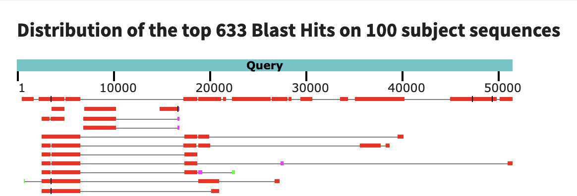
Possibly, the top hit is matching only to the genes of this contig. According to this paper, Immundisolibacter cernigliae is a soil microbe, so we wouldn’t really expect to find it in the ocean. Based on these results, it seems like this nitrogen-fixing population in N06 could be a novel microbe! At the very least, it is not that similar to anything in this database. We are drawing this conclusion based on only one contig sequence from its genome, but even if the rest of its (yet unbinned) genome was similar to that of another microbe in the NCBI database, the fact that this population contains a contig with a near-complete set of nif genes means that it is already substantially different from that hypothetical similar population.
BLAST results for sample N07
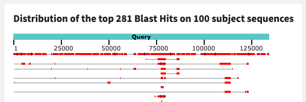
Next, we will view the BLAST results for contig c_000000000073 from sample N07. This contig had all 6 of our nif genes on it.

It has a much better hit in the NCBI database than the previous contig - 85% query coverage with 88% identity. Atelocyanobacterium thalassa is actually a well-known cyanobacterial marine diazotroph (Thompson 2012). Judging by the alignment, N07’s nitrogen-fixing population is extremely similar to this one:
This does not mean that the N07 population resolves to the same taxonomy as A. thalassa - we would need to bin the population and look at the whole genome average nucleotide identity (ANI) as well as other evidence to verify that. But it is similar enough to indicate that this population is not entirely novel.
You might recall that sample N07 had another set of these genes split across a few different contigs. I wonder what you would find if you blasted those? ;)
BLAST results for sample N22
In sample N22, the contig with the most nif genes was c_000000000122. The BLAST results for this contig are below.
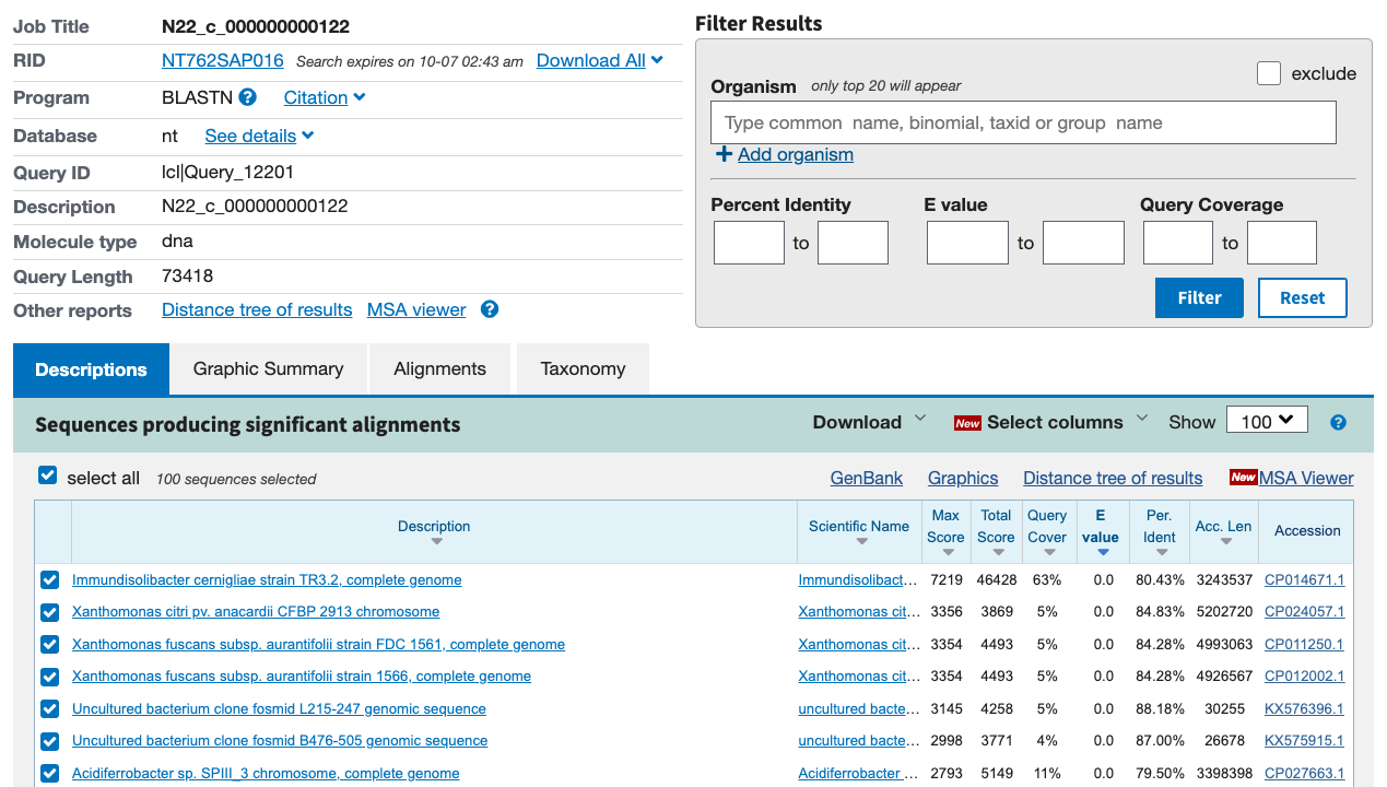
And here is the alignment:
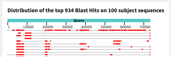
Huh. Just like in N06, the best hit is to the I. cernigliae genome, with somewhat sporadic alignment.
BLAST results for sample N25
The contig from sample N25 gives us extremely similar BLAST results as the one from sample N22:

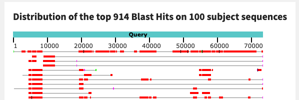
There is a pattern emerging here. Three of the contigs that we’ve looked at thus far have hits to I. cernigliae with similar alignment coverage and identity. It is possible that these three sequences could belong to the same microbial population, in different samples.
To verify their similarity, let’s align the contig sequences to each other.
Aligning N06_c_000000000415 and N25_c_000000000104
The BLAST results for the contigs from N22 and N25 were so similar that we don’t really need to align these two sequences, but the contig from N06 was somewhat different, with only 55% query coverage to the I. cernigliae genome. Let’s align c_000000000415 from N06 and c_000000000104 from N25 to see whether they are similar enough to belong to the same population genome.
I again used the BLAST web service for this, just so I could show you the nice graphical alignment, but feel free to use whatever local sequence alignment program you want. If you are using the online blastn suite, however, you should check the box that says ‘Align two or more sequences’ on the input form so that it will do this instead of searching for your sequences in the NCBI database.
Here is the BLAST hit that I got when I aligned N25_c_000000000104 (the longer contig) to N06_c_000000000415.
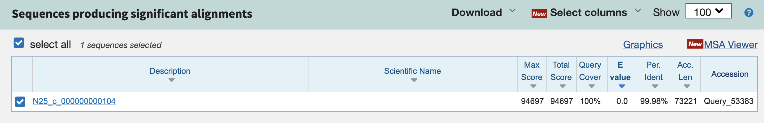
The contigs are extremely similar, with near-100% identity! And the graphical summary shows a long, unbroken alignment:
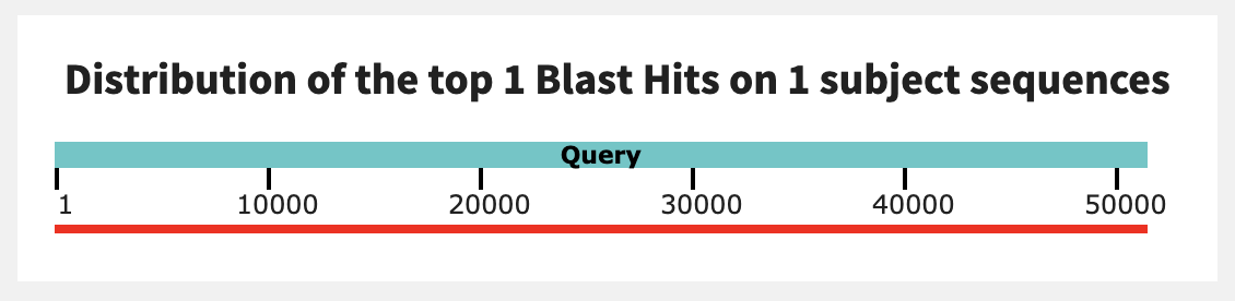
If you were to flip the order of the alignment (aligning the shorter contig from N06 to the longer one from N25), you would get a smaller query coverage value but a similar percent identity. I think these sequences are likely coming from the same microbial population, after all.
Three samples with the same population
This means that at least three of our samples (N06, N22, and N25) have the same nitrogen-fixing microbial population in them. Therefore, if we do read-recruitment of the metagenomes against any one of these samples, we’ll be able to use differential coverage to bin this population.
If you are curious about where these samples are located geographically, here is the sampling map from Figure 1 of the Cao et al. paper, with our three samples highlighted and labeled in purple:
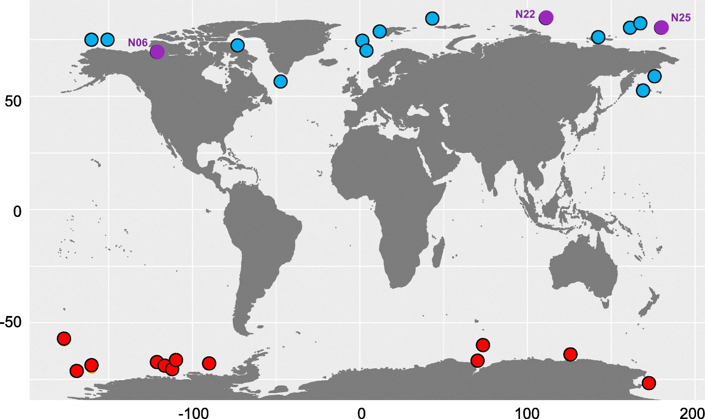
Clearly, this microbial population is widespread in the Arctic Ocean since is found in both the Eastern and Western hemispheres. It also makes sense that the sequences from N22 and N25 are more similar to each other than to the one from N06, since those two samples are geographically closer together.
Comparison of nifH genes
We’ve found a nitrogen-fixing population that appears to be novel, based on its lack of good matches in NCBI. But NCBI is by no means the only source of publicly-available genomic data, so this perhaps does not mean as much as we want it to. To further verify the novelty of this population (while keeping the workload reasonably easy for us), we’re going to check its nifH alignment against other known nifH genes.
When I was doing this analysis, I got a great deal of help from Tom Delmont. He kindly took the nifH gene from contig N25_c_000000000104 and placed it on a phylogeny of known nifH sequences from all around the world (most of them, as you may tell from the phylogeny, come from the TARA Oceans dataset):
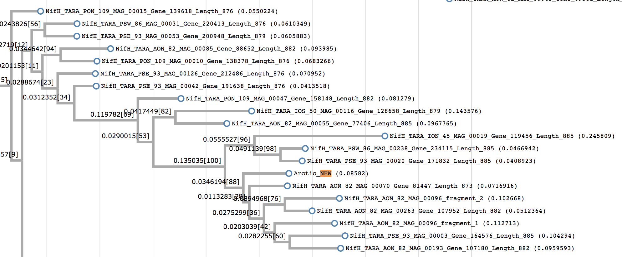
Our population’s nifH was most closely related to nifH genes from the north Atlantic Ocean, but on its own branch, indicating that there are no nifH genes in Tom’s collection that are exactly like it.
However, Tom found that it was most similar (with 95% identity) to the nifH gene from the genome of “Candidatus Macondimonas diazotrophica”, a crude-oil degrader isolated from a beach contaminated by the Deepwater Horizon oil spill (Karthikeyan 2019).
We’re going to check how similar our population is to this “Ca. M. diazotrophica” genome by aligning the N25_c_000000000104 contig against it.
# download the genome
curl -LO http://enve-omics.ce.gatech.edu/data/public_macondimonas/Macon_spades_assembly.fasta.gz
gunzip Macon_spades_assembly.fasta.gz

# extract N25_c_000000000104 sequence into its own file
grep -A 1 "N25_c_000000000104" contigs_of_interest.fa > N25-c_000000000104.fa

# make a blast database for the genome
makeblastdb -in Macon_spades_assembly.fasta \
            -dbtype nucl \
            -title M_diazotrophica \
            -out M_diazotrophica

# run the alignment
blastn -db M_diazotrophica \
       -query N25-c_000000000104.fa \
       -evalue 1e-10 \
       -outfmt 6 \
       -out c_000000000104-M_diazotrophica-6.txt
Looking at the c_000000000104-M_diazotrophica-6.txt file, you should see that the alignments are not very long (the contigs are far longer) and that the percent identities, while high, are not that high.
Here are the top 10 hits in this file:
| qseqid | sseqid | pident | length | mismatch | gapopen | qstart | qend | sstart | send | evalue | bitscore |
|---|---|---|---|---|---|---|---|---|---|---|---|
| c_000000000104 | NODE_14_length_74635_cov_31.4532 | 90.375 | 3761 | 313 | 37 | 19256 | 22978 | 20209 | 23958 | 0.0 | 4894 |
| c_000000000104 | NODE_14_length_74635_cov_31.4532 | 97.212 | 1578 | 43 | 1 | 28370 | 29947 | 63748 | 62172 | 0.0 | 2669 |
| c_000000000104 | NODE_14_length_74635_cov_31.4532 | 77.627 | 3902 | 763 | 93 | 37011 | 40854 | 58320 | 54471 | 0.0 | 2268 |
| c_000000000104 | NODE_14_length_74635_cov_31.4532 | 78.256 | 814 | 141 | 25 | 26446 | 27253 | 67539 | 66756 | 4.59e-137 | 490 |
| c_000000000104 | NODE_14_length_74635_cov_31.4532 | 96.970 | 264 | 8 | 0 | 27955 | 28218 | 64008 | 63745 | 3.62e-123 | 444 |
| c_000000000104 | NODE_14_length_74635_cov_31.4532 | 87.831 | 189 | 23 | 0 | 14301 | 14489 | 72993 | 72805 | 1.85e-56 | 222 |
| c_000000000104 | NODE_11_length_97838_cov_34.3382 | 92.602 | 2379 | 163 | 7 | 4577 | 6948 | 8342 | 5970 | 0.0 | 3406 |
| c_000000000104 | NODE_11_length_97838_cov_34.3382 | 93.967 | 1558 | 92 | 2 | 7018 | 8574 | 5870 | 4314 | 0.0 | 2355 |
| c_000000000104 | NODE_11_length_97838_cov_34.3382 | 81.016 | 748 | 130 | 12 | 13461 | 14203 | 1950 | 1210 | 2.05e-165 | 584 |
| c_000000000104 | NODE_20_length_33832_cov_39.6157 | 82.974 | 417 | 51 | 12 | 72822 | 73221 | 11136 |
While their nifH genes may be very similar, this is certainly not the same population as the one we found.
There is one more set of genes that we should check. In July 2021, Karlusich et al published a paper containing, among other things, a set of 10 novel nifH genes. You will find these genes in the datapack, in the file FASTA/Karlusich_novel_nifH.fa. Make a blast database out of the contig from N25 (which you extracted above), and align these nifH genes against that database.
makeblastdb -in N25-c_000000000104.fa \
            -dbtype nucl \
            -title N25-c_000000000104 \
            -out N25-c_000000000104
blastn -db N25-c_000000000104 \
       -query Karlusich_novel_nifH.fa \
       -evalue 1e-10 \
       -outfmt 6 \
       -out novel_NifH-N25_c_000000000104-6.txt
There are only three hits in the resulting file, and their maximum percent identity is about 86%, so none of them originate from our Arctic Ocean diazotroph.
| qseqid | sseqid | pident | length | mismatch | gapopen | qstart | qend | sstart | send | evalue | bitscore |
|---|---|---|---|---|---|---|---|---|---|---|---|
| ENA MW590317 MW590317.1 | c_000000000104 | 85.000 | 320 | 45 | 2 | 1 | 320 | 4700 | 5016 | 1.97e-90 | 322 |
| ENA MW590318 MW590318.1 | c_000000000104 | 84.211 | 323 | 51 | 0 | 1 | 323 | 4700 | 5022 | 3.26e-88 | 315 |
| ENA MW590319 MW590319.1 | c_000000000104 | 85.802 | 324 | 46 | 0 | 1 | 324 | 4700 | 5023 | 4.16e-97 | 344 |
# navigate out of the FASTA/ folder
cd ..
Identifying the associated Cao et al. MAG
At this point, we’ve verified (to the best of our current knowledge), that we’ve identified an uncharacterized diazotrophic population in these Arctic Ocean metagenomes. Since this novel nitrogen-fixing population is present in multiple samples from the Cao et al. paper, it is extremely likely that the authors have already binned it in some form. So before we bin this population ourselves, we are going to see what else we can learn about it from their data.
Cao et al. did their binning iteratively by running first MaxBin2 and then MetaBAT on the contigs of individual MEGAHIT assemblies of these samples, and they got 214 MAGs out of this process.
We’re going to find out which one of those MAGs represents the nitrogen-fixing population that we have identified in samples N06, N22, and N25. First, download their MAG set, which is hosted on FigShare. You’ll need to unzip the folder, and probably re-name it something sensible (I called the folder Cao_et_al_MAGs, and you’ll see it referred to this way in the code snippets below).
If you don’t want to download all of these MAGs, you can still run an alignment against them using the BLAST database that is in the datapack. You’ll find those files in the CAO_BLAST_DB/ folder (and will either need to move them or change the path to them in the code snippets below).
Each MAG is in a FASTA file that is named according to the MAG number. We will run BLAST against all of these MAGs at the same time, so each MAG’s contig sequences need to have the corresponding MAG number in the contig name. That way we will be able to determine which MAG each BLAST hit belongs to. anvi-script-reformat-fasta is the perfect tool for this job.
The loop in the following code learns the MAG number from its FASTA file name and runs anvi-script-reformat-fasta, which will simplify the contig names and make sure each one is prefixed with the MAG number. The reformatted FASTA files will end in *reformat.fa and the text file matching the original contig name to its new one will end in *reformat_report.txt.
# download Cao et al MAG set
mkdir Cao_et_al_MAGs
cd Cao_et_al_MAGs/
curl -L "https://figshare.com/ndownloader/articles/10302425?private_link=fd5f60b5da7a63aaa74b" -o Cao_et_al_MAGs.zip
unzip Cao_et_al_MAGs.zip
cd ..

# reformat contig names to contain MAG number
for g in Cao_et_al_MAGs/*.fasta; do \
  mag=$(basename $g | sed 's/.fasta//g'); \
  filename=$(echo $g | sed 's/.fasta//g'); \
  anvi-script-reformat-fasta  -o ${filename}_reformat.fa --simplify-names --prefix $mag -r ${mag}_reformat_report.txt $g; \
done

# organize the resulting files into sensible folders
mkdir REFORMAT_REPORTS
mv *reformat_report.txt REFORMAT_REPORTS/
mkdir CAO_MAGS_REFORMATTED
mv Cao_et_al_MAGs/Genome*reformat.fa CAO_MAGS_REFORMATTED/
After that finishes, you can concatenate all of the MAG FASTAs into one big FASTA file, and make a BLAST database out of it:
# concatenate all MAG contigs into one file
cat CAO_MAGS_REFORMATTED/*.fa > all_Cao_MAGs.fa

# make database for mapping against these contigs
makeblastdb -in all_Cao_MAGs.fa \
            -dbtype nucl \
            -title all_Cao_MAGs \
            -out all_Cao_MAGs
Since we know that contigs N06_c_000000000415, N22_c_000000000122, and N25_c_000000000104 are all similar, we only need to BLAST one of them against this database. I chose N25_c_000000000104 arbitrarily, but feel free to try one of the others if you’d like.
# extract sequence into its own file (if you haven't done this already)
grep -A 1 "N25_c_000000000104" FASTA/contigs_of_interest.fa > FASTA/N25-c_000000000104.fa

# blast this contig against all Cao et al MAGs
    # standard output format
blastn -db all_Cao_MAGs \
       -query FASTA/N25-c_000000000104.fa \
       -evalue 1e-10 \
       -out c_000000000104-all_Cao_MAGs-0.txt
    # tabular output format
blastn -db all_Cao_MAGs \
       -query FASTA/N25-c_000000000104.fa \
       -evalue 1e-10 \
       -outfmt 6 \
       -out c_000000000104-all_Cao_MAGs-6.txt
If you look at the tabular output file, you will see that there is really only one good match for contig N25_c_000000000104, and that is a hit against Genome_122_000000000019 (or, contig 19 from Genome_122. The reformat report for this MAG indicates that contig 19 was originally named k141_74885. In case that matters to anyone.). It has almost 100% identity over nearly the entire contig (you can see the alignment in the standard output file, if you are curious about that).
It seems like Genome_122 is the nitrogen-fixing MAG that we have been looking for. In fact, supplementary table S5 from the Cao et al. paper indicates that (according to GTDB-Tk) this MAG belongs to the Immundisolibacter genus. Well, we have seen enough of the alignments to know that this taxonomy is probably not correct, but it was the closest match on NCBI. This is enough to verify that we found the correct MAG.
So a MAG of our population of interest has already been binned, as expected. If this weren’t a blog post on how to do targeted binning, you might think that we were done here. But it is a blog post about targeted binning, so we are not done just yet. :) We will do our own binning in just a moment. In the meantime, we can still use the Cao et al. MAG to learn things about our population of interest that will help us bin this population ourselves - namely, the distribution of this population in different parts of the ocean, which will help us know what to expect in terms of differential coverage patterns.
In addition, this Genome_122 MAG was binned automatically without any manual refinement, which as we know can be problematic. Is this MAG complete? Is it chimeric? As we investigate it further in the next section, keep these questions in mind, because their answers will further motivate us to bin this population ourselves.
Distribution of Genome_122 in the global oceans
Thus far, we’ve 1) identified a nitrogen-fixing population in the Arctic Ocean, 2) inferred its novelty from its lack of matches to NCBI and a collection of known nifH genes, and 3) found its corresponding MAG in the Cao et al. data. Our next question is - where does this population occur across the world? Can it be found only in the Arctic, or is it a globally-distributed population (that for some reason has not yet been characterized in temperate oceans)? Is it limited to the surface ocean, or can it live in the deep?
To answer this question, I mapped four different datasets of ocean metagenomes to the Genome_122 MAG using the anvi’o metagenomic workflow. Those datasets are: the current one from Cao et al. (including all samples, from the Arctic and Antarctic), the ACE dataset of Southern Ocean metagenomes (which is yet unpublished, but is a sampling expedition led by our collaborator Lois Maignien at the IUEM-Brest), and the vast global ocean sampling efforts TARA and TARA2. We’re going to look at these mapping results. You will find the relevant databases in your datapack, in the GENOME_122_DBS folder.
Surface ocean distribution
First, open up the anvi’o interactive interface and take a look at the distribution of this MAG in the surface ocean (which includes metagenomes sampled at depths 0-100m from these four datasets):
cd GENOME_122_DBS/
anvi-interactive -c Genome_122-contigs.db \
                 -p SURFACE/SURFACE_PROFILE.db \
                 --title "Genome_122 in Surface Ocean"
You should see something like the following:
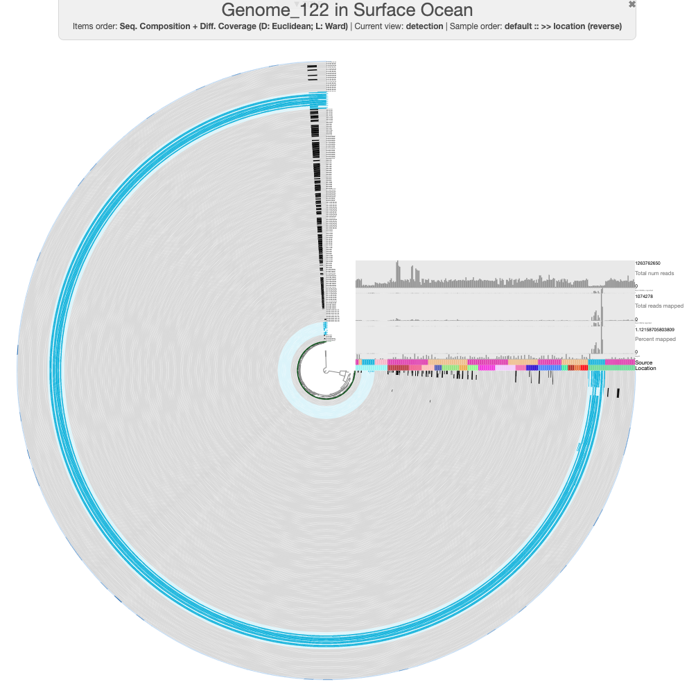
The default view in the interface should show log-normalized detection of this MAG in all of the ocean metagenomes. Each concentric circle in the figure is one metagenome sample, and each spoke of the wheel is a contig from GENOME_122. Samples from Cao et al. have been marked in light blue to distinguish them from the rest. You can hover over the ‘Source’ layer to see which dataset each sample comes from, and the ‘Location’ layer to see which ocean region it was sampled from.
There are a few things we can immediately see from the mapping results. First, it is clear that this population is geographically isolated, as it is detected only in the Arctic Ocean samples from the Cao et al. dataset. There are some Arctic Ocean samples from TARA2 (the darkest green in the ‘Location’ layer), but this population is not detected in these. Second, this MAG must have been binned from the Cao et al. assembly of sample N07, since that sample has the highest proportion of mapping reads. Though we didn’t discuss it earlier, our nitrogen-fixing population is also present in sample N07 (which you may already have deduced if you took a look at the BLAST results for the second set of nif contigs in N07).
Finally, there are several splits in Genome_122 that appear to be contamination. For instance, look at these three splits that have different detection values across samples than the rest of the MAG:
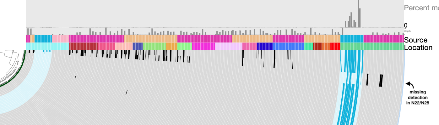
One of those splits is missing detection in samples N22 and N25 (where we know our population exists) - this split is marked with an arrow in the figure above. The other two are detected in a variety of samples from the other datasets as well as a different detection pattern across the other Cao et al. Arctic Ocean samples. There are also a couple more splits at the top of the circlular phylogram that seem problematic.
A quick aside to look for nif genes
Recall that contig 19 from this MAG is the one most similar to the contig from sample N25 that we blasted earlier, which means it should be the contig containing most of the nif genes we were looking for. Can you find this contig and/or the nif genes? (hint: use the ‘Search’ tab)
Well, I’m sure you found contig 19. But you couldn’t find our nif genes, could you? In fact, if you search for functions with “nitrogen fixation”, you will find several annotated nif genes but not the ones that we were looking for - except for nifB, which is not on contig 19 (as expected) but on contig 27. This is extremely curious. How could this happen? Previously, contig N25_c_000000000104, which contains 5 out of 6 of our nif genes, matched with almost 100% identity against the entirety of contig 19 - so what is missing?
It turns out that contig 19 is quite a bit shorter - only 51,626 bp - compared to N25_c_000000000104’s length of 73,221 bp. You might have noticed this if you checked the standard output file from BLAST. Clearly, the part of contig 104 that contains those 5 nif genes was not the part that matched to contig 19. We are working with different assemblies of these metagenomes than the ones created by Cao et al., so some differences are to be expected.
Furthermore, we now know that Genome_122 was binned from sample N07. In N07, the second set of nif genes was split across 3 contigs (c_000000004049, c_000000000256, and c_000000000095), so it is likely that a similar situation occurred in the Cao et al. assembly of this sample. Which means it is certainly possible that only the contig containing nifB was binned into this MAG. Contig 27 from Genome_122 is probably the counterpart to c_000000000095 from our assembly.
You can check this, if you want, by blasting those three N07 contigs against the Cao et al. MAGs:
# go back to the previous folder
cd ..

# extract just these 3 contigs from N07 into a separate file
for c in c_000000004049 c_000000000256 c_000000000095; \
do \
  grep -A 1 $c FASTA/contigs_of_interest.fa >> FASTA/N07_second_set.fa; \
done

# align against the MAG set
blastn -db all_Cao_MAGs \
       -query FASTA/N07_second_set.fa \
       -evalue 1e-10 \
       -outfmt 6 \
       -out N07_second_set-all_Cao_MAGs-6.txt
I’ll paste the relevant hits from the output below. These are the best hits for each contig query (meaning that they have the highest percent identity, the longest alignment lengths, and the smallest e-value of all hits from that contig):
| qseqid | sseqid | pident | length | mismatch | gapopen | qstart | qend | sstart | send | evalue | bitscore |
|---|---|---|---|---|---|---|---|---|---|---|---|
| N07_c_000000000095 | Genome_122_000000000027 | 99.982 | 116075 | 5 | 5 | 1 | 116072 | 116114 | 43 | 0.0 | 2.142e+05 |
| N07_c_000000004049 | Genome_022_000000000007 | 99.729 | 7751 | 20 | 1 | 92 | 7841 | 14062 | 6312 | 0.0 | 14196 |
| N07_c_000000004049 | Genome_022_000000000007 | 99.203 | 753 | 6 | 0 | 7824 | 8576 | 2534 | 1782 | 0.0 | 1358 |
| N07_c_000000000256 | Genome_122_000000000019 | 99.992 | 51584 | 4 | 0 | 13380 | 64963 | 51626 | 43 | 0.0 | 95236 |
First of all, contig N07_c_000000000095 (the one with the nifB gene) indeed matches extremely well to contig 27 from Genome_122, as expected. Contig N07_c_000000004049, which contained a copy of the M00175 module, does not match to anything in Genome_122 at all (which explains why those three genes were missing from the MAG). Instead it matches to a contig from the MAG named Genome_022, but the alignment length is rather small.
However, contig N07_c_000000000256, which contained nifE and nifN in our assembly, matches to contig 19 of Genome_122! It is 64,963 bp long, so here we have the same situation as contig 104 from sample N25 - it is a much longer sequence than contig 19, and the nifE and nifN genes must be on the part that does not match to contig 19. (Indeed, if you blast N07_c_000000000256 against N25_c_000000000104, it will match to one end of that contig.)
The long story short is that our nif genes of interest were not binned into the Genome_122 MAG, but we have plenty of evidence that they do belong to this population, considering that those genes were assembled together in other samples. Sadly, that means that Genome_122 is incomplete, and it is missing the genes we care most about. But more on this later.
Deep ocean distribution
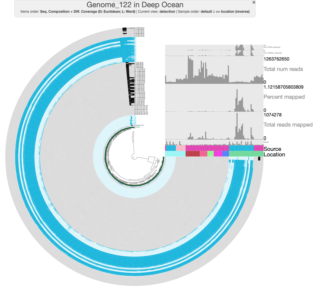
The next thing to view is the distribution of this MAG in deeper samples (100m < depth <= 3800 m).
cd GENOME_122_DBS/
anvi-interactive -c Genome_122-contigs.db \
                 -p DEEP/DEEP_PROFILE.db \
                 --title "Genome_122 in Deep Ocean"
The samples are color-coded in the same way as before. You should be able to see that this MAG is present in deeper waters (even those as deep as 3800m), though it is still geographically limited to the Arctic Ocean. And once again, there are several splits that just don’t seem to fit with the rest and most likely represent contamination.
Are you interested in the taxonomy of this MAG? I bet you already have a guess as to what it is, considering what we’ve seen so far. :) But if you want to check it, you can run the following code to find out what anvi’o thinks its taxonomy is:
anvi-estimate-scg-taxonomy -c Genome_122-contigs.db
# we are done here, go back to parent directory
cd ..
Targeted binning of the nitrogen-fixing population
We’ve seen above that the Genome_122 MAG appears to have some contamination, which is a normal thing to see in MAGs (particularly automatically-generated ones), because binning is hard. We’ve also seen that it does not contain the nif genes that belong to this nitrogen-fixing population. But since we have time on our hands, a particular interest in just this one nitrogen-fixing population, and the knowledge of which nif gene-containing contigs belong to this population, we can make a better MAG. It’s time for some targeted binning. :)
We know that our population of interest is present in samples N06, N07, N22, and N25. We could use any of these assemblies for binning, though N07 is not the best choice because the nif genes are split across more contigs in that one. I once again made the completely arbitrary choice to use sample N25 for this. I ran a read recruitment workflow to map all 60 Cao et al. metagenomes against our assembly of N25 so that we can look at differential coverage across different metagenomes- our population of interest should only be present in the Arctic Ocean samples, but we will be able to use its absence from the Antarctic samples to help guide our binning.
You’ll find the contigs database for the N25 assembly and the profile database containing these mapping results in the datapack (in the N25_DBS folder). You can open them up in anvi-interactive:
cd N25_DBS/
anvi-interactive -c N25-contigs.db \
                 -p PROFILE.db \
                 --title "Cao et al Read Recruitment to N25" \
                 --state-autoload binning
The databases are rather large, and may take some time to load, but once they do you should see the following display:
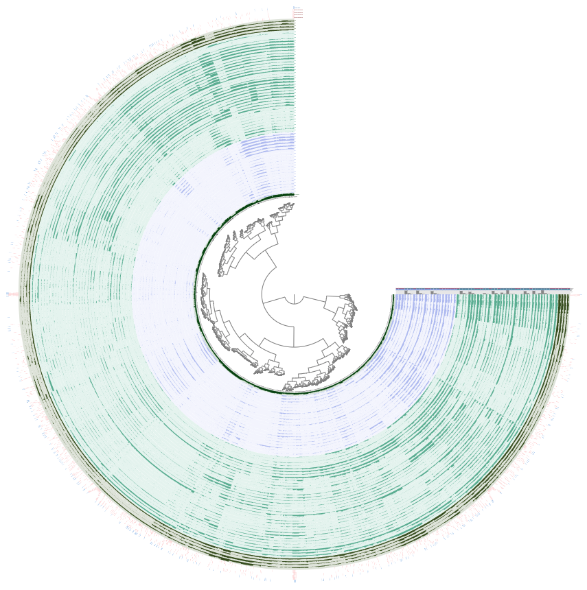
The Arctic Ocean samples are green, and the four samples we expect to find our population in are the outermost, darker green layers so that we can more easily focus on those. The blue samples are the Antarctic ones.
We will start our binning with the contig that contains the most nif genes in N25, which is 000000000104. You can search for this contig in the ‘Search’ tab of the ‘Settings’ panel, and add its splits to a bin.
The contigs in this assembly are clustered according to their sequence composition and their differential coverage (across all Cao et al. samples), so the other contigs that belong to our nitrogen-fixing population should be located next to contig 000000000104 in the circular phylogram. These contigs should also appear in all four of our samples of interest (dark green), have zero coverage in the Antarctic samples (blue), and have similar GC content (the green layer below the Antarctic samples). If you zoom to the location of the splits you just binned, you should see a set of splits that fit this criteria.
Did you find it? Here are the splits I am talking about, so you can check your work:
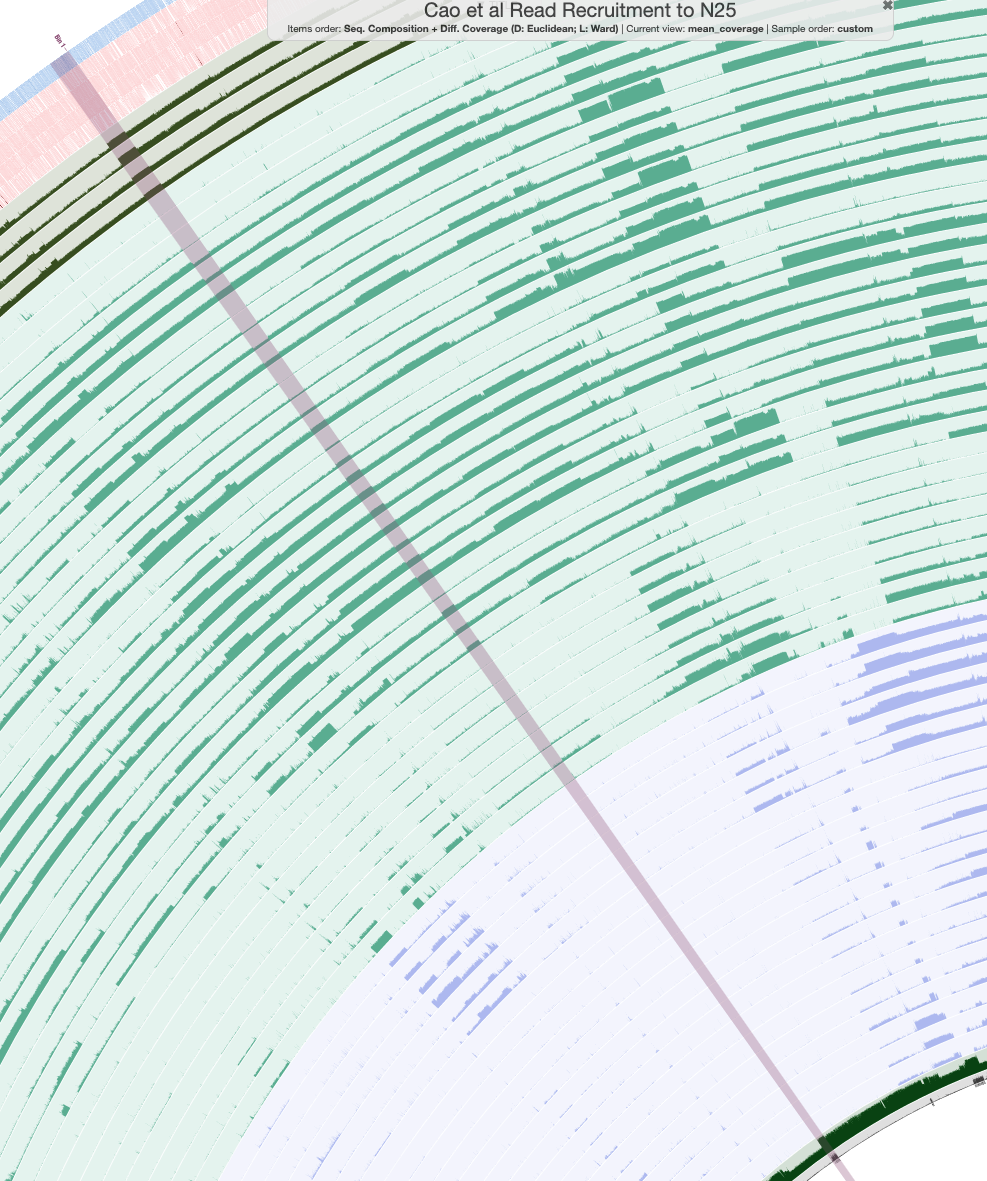
These were the splits that I binned (there are 168 of them). You can bin them yourself, or just load the collection called Nif_MAG to see the same bin on your own screen. The anvi’o estimates of completion and redundancy (based on bacterial single-copy core genes) for this bin are 100% and 0%, respectively, which is great news. Furthermore, if you check the box for real-time taxonomy estimation on the “Bins” tab, you will see that this bin is labeled as Immundisolibacter cernigliae, the same microbe that we kept getting BLAST hits to previously. So we’ve certainly binned the correct population, and it is a high-quality MAG at that.
Bonus activity: Recall that there were 3 copies of the NifB in sample N25, on three separate contigs. Which one belongs to this population?
Estimating metabolism for our new MAG
Now that we have a complete MAG for our nitrogen-fixing population, let’s see what else it can do. We are going to run metabolism estimation on this population.
There are a couple of different ways we can go about this. Since the bin is saved as a collection, you can directly estimate its metabolism from the current set of databases for the entire N25 assembly, just like this:
anvi-estimate-metabolism -c N25-contigs.db \
                         -p PROFILE.db \
                         -C Nif_MAG \
                         -O Nif_MAG \
                         --kegg-output-modes kofam_hits,modules
Or, you could split this MAG into its own set of (smaller) contig/profile databases, and then run metabolism estimation in genome mode:
anvi-split -c N25-contigs.db \
           -p PROFILE.db \
           -C Nif_MAG \
           -o Nif_MAG
anvi-estimate-metabolism -c Nif_MAG/Nif_MAG/CONTIGS.db \
                         -O Nif_MAG \
                         --kegg-output-modes kofam_hits,modules
You can pick whichever path you like. I went with the latter option because I wanted a stand-alone database for the MAG so I could do other things with it, but the former is less work for you (and for your computer). Regardless of how you do it, you should end up with a Nif_MAG_modules.txt file containing the module completeness scores for this population, and a Nif_MAG_kofam_hits.txt file containing its KOfam hits.
You are free to explore these results according to your interests, but one of my remaining questions about this population is whether it is a cyanobacteria or a heterotroph. Cyanobacteria have photosynthetic and carbon fixation capabilities, while heterotrophs have ABC transporters for carbohydrate uptake (Cheung 2021). I looked for modules related to each of these things and checked their completeness scores.
Here is my search code. I once again clipped the output so that it shows only relevant fields.
head -n 1 Nif_MAG_modules.txt | cut -f 3,4,7,9; \
grep -i "carbon fixation" Nif_MAG_modules.txt | cut -f 3,4,7,9
| kegg_module | module_name | module_subcategory | module_completeness |
|---|---|---|---|
| M00165 | Reductive pentose phosphate cycle (Calvin cycle) | Carbon fixation | 0.8181818181818182 |
| M00166 | Reductive pentose phosphate cycle, ribulose-5P => glyceraldehyde-3P | Carbon fixation | 0.75 |
| M00167 | Reductive pentose phosphate cycle, glyceraldehyde-3P => ribulose-5P | Carbon fixation | 0.8571428571428571 |
| M00168 | CAM (Crassulacean acid metabolism), dark | Carbon fixation | 0.5 |
| M00173 | Reductive citrate cycle (Arnon-Buchanan cycle) | Carbon fixation | 0.8 |
| M00376 | 3-Hydroxypropionate bi-cycle | Carbon fixation | 0.4423076923076923 |
| M00375 | Hydroxypropionate-hydroxybutylate cycle | Carbon fixation | 0.14285714285714285 |
| M00374 | Dicarboxylate-hydroxybutyrate cycle | Carbon fixation | 0.38461538461538464 |
| M00377 | Reductive acetyl-CoA pathway (Wood-Ljungdahl pathway) | Carbon fixation | 0.2857142857142857 |
| M00579 | Phosphate acetyltransferase-acetate kinase pathway, acetyl-CoA => acetate | Carbon fixation | 0.5 |
| M00620 | Incomplete reductive citrate cycle, acetyl-CoA => oxoglutarate | Carbon fixation | 0.35714285714285715 |
Several of the reductive pentose phosphate cycle pathways look near-complete. However, these results must be taken with a grain of salt because many of these pathways share a large number of their KOs with other pathways. We can confirm whether or not this is a cyanobacteria by looking for photosynthesis capabilities:
head -n 1 Nif_MAG_modules.txt | cut -f 3,4,7,9; \
grep -i "photo" Nif_MAG_modules.txt | cut -f 3,4,7,9
| kegg_module | module_name | module_subcategory | module_completeness |
|---|---|---|---|
| M00532 | Photorespiration | Other carbohydrate metabolism | 0.475 |
| M00611 | Oxygenic photosynthesis in plants and cyanobacteria | Metabolic capacity | 0.4090909090909091 |
| M00612 | Anoxygenic photosynthesis in purple bacteria | Metabolic capacity | 0.4090909090909091 |
| M00613 | Anoxygenic photosynthesis in green nonsulfur bacteria | Metabolic capacity | 0.22115384615384615 |
| M00614 | Anoxygenic photosynthesis in green sulfur bacteria | Metabolic capacity | 0.4 |
As you can see, none of these modules are complete (including the pathway specifically for cyanobacteria), so this doesn’t appear to be a cyanobacterial population. A huge caveat here is that our MAG could simply be missing the genes relevant to this pathway (or, it has them, but they are not homologous enough to their corresponding KO families to be annotated). This is a possibility with any MAG. But if we choose to trust these estimations (given the high completeness score of our bin), the current evidence points to this population being heterotrophic.
There is no module for carbohydrate transporters, since these are individual proteins rather than a metabolic pathway, but we can look for KOfam hits that are annotated as transporters instead.
head -n 1 Nif_MAG_kofam_hits.txt | cut -f 3-5,7; \
grep -i 'transport' Nif_MAG_kofam_hits.txt | cut -f 3-5,7
There are plenty of hits, including several specifically for carbohydrates:
| ko | gene_caller_id | contig | ko_definition |
|---|---|---|---|
| K16554 | 16040 | N25_000000000138 | polysaccharide biosynthesis transport protein |
| K02027 | 21931 | N25_000000000271 | multiple sugar transport system substrate-binding protein |
| K02026 | 21933 | N25_000000000271 | multiple sugar transport system permease protein |
| K02025 | 21932 | N25_000000000271 | multiple sugar transport system permease protein |
| K10237 | 21932 | N25_000000000271 | trehalose/maltose transport system permease protein |
| K10236 | 21931 | N25_000000000271 | trehalose/maltose transport system substrate-binding protein |
| K10238 | 21933 | N25_000000000271 | trehalose/maltose transport system permease protein |
So it looks like this microbe is indeed a heterotroph, which would make it a heterotrophic bacterial diazotroph, or HBD. It can join its temperate ocean relatives in Tom’s hard-earned collection.
Final Words
So there you have it - a novel, heterotrophic nitrogen-fixing population from the Arctic Ocean, binned directly from public metagenomes with a bit of guidance from anvi-estimate-metabolism. We went fishing, and we caught something interesting. And it wasn’t all that hard. :)
If you ever have to look for a microbe of interest in metagenomic data, and you know it has something unique in terms of its metabolic capabilities, you can try out this technique in your search. Perhaps you’ll find what you are looking for!