discov-stats

A TXT-type anvi’o artifact. This artifact is typically generated, used, and/or exported by anvi’o (and not provided by the user)..

🔙 To the main page of anvi’o programs and artifacts.

Provided by

anvi-profile-blitz

Can be provided by

anvi-summarize

Required by

There are no anvi’o tools that require this artifact directly, which means it is most likely an end-product for the user.

Description

The Distribution of Coverage (DisCov) score is designed to capture the presence-absence of a contig or genome (‘bin’) in a metagenomic sample, as an alternative to using arbitrary detection thresholds for this purpose. DisCov quantifies how well a sequence is covered by reads — not just how many bases have coverage, but whether that coverage is spread across the sequence and whether it is roughly even in depth. To achieve this, DisCov incorporates two independent metrics:

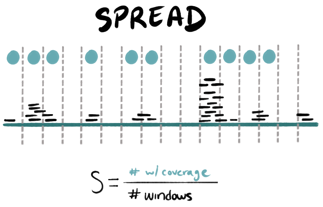
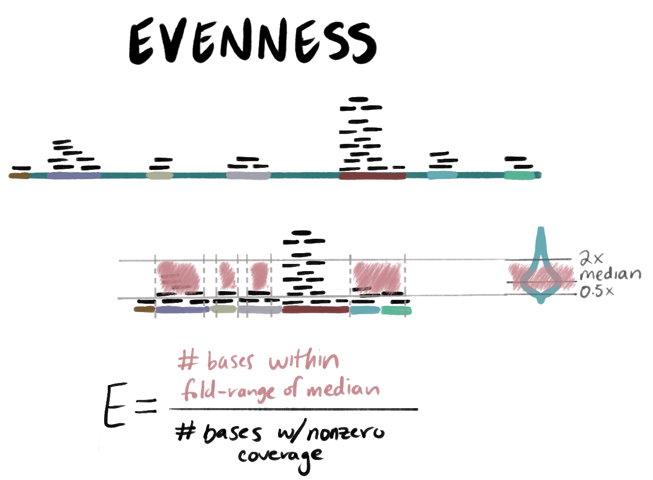
• S (spread): the proportion of non-overlapping windows across the sequence that include bases with at least 1X coverage. In other words, S = # of windows with coverage / # of windows.
• E (evenness): the proportion of covered bases whose coverage falls within an expected fold-range of the median nonzero coverage. In other words, E = # covered bases that fall within some range of the median / # of covered bases

These are combined into a single score using either a linear or geometric formula:

• Linear: DisCov = αS + (1-α)E
• Geometric: DisCov = S^α × E^(1-α)

where α is a value between 0 and 1 that controls how much weight is given to spread (S) relative to evenness (E). By default α = 0.5 (equal weighting) and the linear formula is used, so DisCov is simply the average of S and E.

When DisCov values are reported – for instance, in bam-stats-txt – usually S, E, and the number of windows are individually reported in addition to the overall DisCov score.

Technical details & parameters

Here you’ll find a description on how DisCov is computed. You can modify most aspects of the DisCov calculation, and the parameters for each step are mentioned when relevant below.

Programs that produce these stats

anvi-profile-blitz always computes DisCov scores as part of its output. anvi-summarize computes DisCov scores when the --report-discov flag is provided.

Input data

S, E, and DisCov scores are computed based on per-nucleotide coverage arrays for individual contigs. When computing scores at the genome-level, the arrays for all contigs within a given genome (or more generically, a given bin) are concatenated. Note that the concatentation of per-contig coverage arrays means that the windows for the S metric can span across contig boundaries within the genome.

The per-base coverage arrays are either obtained directly from a bam-file, or from the auxiliary database files (AUXILIARY-DATA.db) produced by anvi-profile.

S and window length

We divide each sequence (contig or genome) into non-overlapping windows to compute S. S is therefore essentially a more coarse-grained version of the regular detection metric (proportion of bases with coverage), and the window size affects its sensitivity. We want the windows to be long enough to capture meaningful clusters of mapped reads (hence, longer than typical short-read lengths), but short enough to effectively assess the distribution of these mapped reads along the sequence.

There are two strategies for setting the window length:

• Fixed window length (--window-length): a constant window size in bp applied to all sequences.
• Percentage-based window length (--window-length-as-percentage): the window size is set as a percentage of each sequence’s length, optionally with a minimum length floor (--min-window-length).

If you don’t explicitly set any of these parameters, the default sizing strategy depends on the context. For genome-level stats, the default is a fixed 1,000 bp window. For contig-level stats, a percentage-based window (1% of contig length, with a minimum of 300 bp) is used to better accommodate contigs of varying sizes.

If a contig (or genome) is shorter than the window length, the sequence will not be divided; that is, the entire sequence will be a single window. In this case, the S metric collapses to a binary value (does the sequence have any coverage, or not), and from there: (1) If the sequence has no coverage at all (S = 0), DisCov will be 0 (as the evenness metric E will also be 0). (2) If the sequence does have coverage (S = 1), then the DisCov value will have a minimum value of α and the increase from α is determined by E: DisCov = α + (1-α)E. DisCov may not be very meaningful for these short sequences. In most cases, anvi’o will warn you if sequences are shorter than the computed window length, and regardless you should be able to see the number of windows per sequence in the output files.

Removal of very short ‘remainder’ windows

Since the windows for computing S are non-overlapping, the final window in the sequence is often shorter than the other windows (its length is the remainder when you divide the total sequence length by the window size). In general it is not a big problem to include one shorter window in the calculation, but it means that these final bases can sometimes have very disproportional representation in the spread metric. So when the remainder is very small (<10% of the window size), we exclude the final, shorter window entirely from the calculation of S.

What happens if we using a fixed window length and are dealing with very short contigs that by themselves are <10% of that length? We don’t throw anything away, and those contigs will have exactly 1 window.

E and the fold-range

Evenness is computed only based upon the bases with nonzero coverage in the input sequence; that is, we filter the coverage array to keep only the nonzero values. From these nonzero coverage values, we compute the median coverage depth and multiply this value by the fold-range lower and upper bound to establish a range of ‘expected’ coverage depth. Bases with coverage depth within this range are counted as “evenly covered”.

You can adjust the fold-range to accommodate more or less variation in coverage depth by setting --foldrange-lower and --foldrange-upper. Wider fold-range values are more permissive; narrower ones are stricter. The default lower bound is 0.5x the median nonzero coverage while the default upper bound is 2.0x the median nonzero coverage. Note that these values are not required to be inverses of each other; for example, you could set a lower bound of 0.2x and an upper bound of 3x.

The reliance on nonzero coverage values means that E can have extremely high values when few reads map to a sequence. Even if an input sequence is 1,000,000 bp long, if it has only one read of 300 bp mapping to it, E will be computed based upon the subset of ~300 bp where that read maps. In this example, there is an even 1x coverage on every single base of the ~300bp, and therefore E = 1. With the linear DisCov formula and the default α of 0.5, the DisCov score in a situation like this would be 0.5 despite the relative lack of read mapping, due to the high evenness. If that seems like too high of a score for this situation, then you can adjust α or use the geometric formula for DisCov instead to penalize cases where S is very low.

The weight parameter α

You can adjust the weights on S and E by setting the --alpha parameter. Increase α to increase the importance of spread, and decrease α to increase the importance of evenness. α should always be between 0 and 1 (inclusive. In case you really want DisCov to be equivalent to one of S or E you can set α = 1 or α = 0, respectively).

Choosing the DisCov formula

The parameter --discov-formula controls which equation is used to combine S and E into the final DisCov score. If it’s linear (the default), we take a weighted average of S and E, and if it’s geometric, we compute a weighted geometric mean of the two.

Each formulation has pros and cons. The linear version is typically easier to interpret – high numbers mean at least one of S and E is high and this often is a good evidence for presence in a metagenome sample. However, the exceptions to this are the edge cases mentioned in the warning boxes above – S will be 1.0 for very short input sequences with some coverage while E will be 1.0 when a few isolated reads map to the sequence. Those cases yield mid-level DisCov scores even though the evidence for their presence is not very strong, and that means that linear DisCov values close to ~0.5 are rather ambiguous (they might result from similar yet low-ish values of S and E, or they might result from these extreme edge cases where one takes a value near 1.0 and the other takes a value near 0.0). The alternative geometric formulation requires input sequences to have both high S and high E to yield a high DisCov score and can therefore more clearly distinguish ambiguous cases.

Still not sure which formulation is best for your data? You could always compute both and maybe even combine them :)

Okay, but how do I use DisCov?

You can use DisCov to decide if a given sequence is present or absent in a metagenome sample by setting a threshold score above which it is considered present. Where you draw the line depends on how confident you want to be (or how much you want to avoid false positives). A rough guideline based on insights during testing: for linear DisCov, don’t use a threshold any lower than ~0.6, and for geometric DisCov, don’t use any threshold lower than ~0.5.

More resources

• The DisCov Pull Request explains some implementation decisions, shows results from the hyperparameter tuning used to set the default parameters, and also describes the outcome of various validation tests.

Edit this file to update this information.