An exercise on metabolic reconstruction in anvi'o

Table of Contents
- Running the metabolism suite of programs - a single-genome example
- Metabolism estimation and enrichment on a real-world dataset
- A dataset of high- and low-fitness MAGs
- Estimating metabolism for these MAGs
- Finding enriched metabolic pathways
- Estimating pathway copy number in a metagenome assembly
- Exploring pathway coverage in metagenomes
- Conclusion
This is a tutorial for the metabolism suite of programs in anvi’o. First, we will learn how to estimate metabolism for a single bacterial isolate, starting from its genome sequence and ending with a file of metabolic module completeness scores. Afterwards, we’ll be applying this to a larger, real-world dataset of metagenome-assembled genomes from our recent FMT study, to learn how to estimate metabolism in a more high-throughput manner as well as how to compute enrichment scores for metabolic modules.
This tutorial is tailored for anvi’o v8 but will probably work for later versions as well (perhaps with minor command modifications). You can learn the version of your installation by running anvi-interactive -v in your terminal.
Running the metabolism suite of programs - a single-genome example
For this example, we’ll be using a bacterial isolate genome from the NCBI - the representative genome for Akkermansia muciniphila. I picked this species because it is a pretty cool gut microbe that can degrade mucin (Derrien 2004). But if you have your own data or an interest in a different species, feel free to use that instead.
Here is how you can download and unpack the A. muciniphila genome:
curl -LO https://ftp.ncbi.nlm.nih.gov/genomes/all/GCF/009/731/575/GCF_009731575.1_ASM973157v1/GCF_009731575.1_ASM973157v1_genomic.fna.gz && \
gunzip GCF_009731575.1_ASM973157v1_genomic.fna.gz
The first step in any anvi’o analysis is to get your data into the form that anvi’o likes to play with, which means we need to make a contigs database. To do this, we first need to re-format the FASTA file to make sure all of the contig deflines contain nothing more than alphanumeric characters, underscores, and dashes. We can do this with anvi-script-reformat-fasta. Then we can pass the reformatted FASTA to anvi-gen-contigs-database and let it work its magic:
# fix the deflines
anvi-script-reformat-fasta GCF_009731575.1_ASM973157v1_genomic.fna \
                          --simplify-names \
                          --output-file A_muciniphila.fa

# convert FASTA into a contigs db
anvi-gen-contigs-database --contigs-fasta A_muciniphila.fa \
                          --project-name A_muciniphila \
                          --output-db-path A_muciniphila-CONTIGS.db \
                          --num-threads 2
The command above sets the --num-threads parameter to 2 so that anvi-gen-contigs-database works a bit faster, but please take care that your computer has enough CPUs to accommodate this number of threads. This applies anytime you see the --num-threads or -T parameter in a command.
Now you have a contigs database for this genome, so we can start to work with it to estimate metabolism. There are 3 required steps in the metabolism estimation process (though the first step is only necessary the very first time you are doing this, so in general there are just 2 steps). Those steps are:
- Getting the required KEGG data set up on your computer (which only needs to be done once) with anvi-setup-kegg-data
- Adding functional annotations from the KOfam database to the gene calls in this genome, using anvi-run-kegg-kofams
- Matching those functional annotations to definitions of metabolic pathways (aka modules) and computing module completeness scores, which is done by the program anvi-estimate-metabolism
You can learn more about how each of these programs work (and different options for running them) by clicking on any of the highlighted links above to go to their respective help pages. Below we will go through a simple example of each step using the A. muciniphila genome that we just downloaded.
Setting up KEGG data on your computer
First, if you’ve never worked with KEGG data through anvi’o before (which is likely, considering what you are reading right now), you will need to get this data onto your computer so that the downstream programs can use it. This is as simple as running the following:
anvi-setup-kegg-data
That’s it. What this does is download a bunch of data from KEGG onto your computer. The data that are relevant to metabolism estimation are: 1) profile hidden Markov models (pHMMs) for functional annotation from the KOfam database and 2) metabolic pathway definition files from the KEGG MODULE database. The pHMMs have been organized into one big file that is ready for running hmmsearch, and the module definitions have been parsed into a modules database. This program also downloads data relevant for metabolic modeling in anvi’o, but we don’t have to worry about that for the purposes of this tutorial.
By default, the KEGG data goes into the anvi’o directory on your computer. If you don’t have permission to modify this folder, you will need to pick a different location (that you do have permission to modify) for the data and specify that folder using the --kegg-data-dir parameter. If this is your case, please note that running anvi-run-kegg-kofams and anvi-estimate-metabolism will also require you to specify that folder location with --kegg-data-dir.
The data that is downloaded by default is actually a snapshot of KEGG at one moment in time in the past, which we downloaded directly from KEGG and pre-processed into formats compatible for downstream anvi’o programs (using this same program). Downloading the snapshot has several benefits. First, we avoid overloading the KEGG servers when multiple people are downloading the data at once. Second, if KEGG ever changes their file formats and breaks our setup code, we can still use the previous snapshots. Third, everyone with the same version of anvi’o uses the same version of KEGG, which makes data sharing and reproducibility easier. You can choose between several snapshots of KEGG, and you can also use anvi-setup-kegg-data to download the data directly from KEGG to get the latest version of data. You can see instructions for doing that here. But for this tutorial, we will assume that you are working with the default snapshot for anvi’o v8 (and the example outputs will reflect that data).
To check that you have the version of KEGG data that matches to the one we are using in this tutorial, you can run the following (assuming that you are using the default KEGG data directory):
# learn where the MODULES.db is:
export ANVIO_MODULES_DB=`python -c "import anvio; import os; print(os.path.join(os.path.dirname(anvio.__file__), 'data/misc/KEGG/MODULES.db'))"`

# print the path so you can see where it is located
echo $ANVIO_MODULES_DB

# check the hash of the MODULES.db contents
anvi-db-info $ANVIO_MODULES_DB
In the ‘DB Info’ output, you should see the following hash value:
hash .........................................: a2b5bde358bb
Different KEGG version?
If your modules-db hash is not matching (for instance, if you are using a different version of anvi’o or have intentionally downloaded a different snapshot or directly from KEGG), then you can get the same version by specifying the snapshot name we are using. In this case, we recommend specifying a new location for the data using --kegg-data-dir to avoid overwriting your default KEGG data directory, and we remind you that you should use --kegg-data-dir to point to that non-default directory in all metabolism-related programs going forward.
Here is how you could do this (you can change the directory name if you want to):
anvi-setup-kegg-data --kegg-snapshot v2023-09-22 --kegg-data-dir ./KEGG_2023-09-22_a2b5bde358bb
Annotating the genome with KOfam hits
The contigs database includes predicted gene calls (open reading frames, or ORFs), but we don’t know what functions these genes encode. The next step is annotating these genes with hits to the KOfam database of functional orthologs. If a gene is similar enough to a protein family in this database, it will be annotated with the family’s KEGG Ortholog (KO) number. This number is what allows us to match genes to the metabolic pathways that they belong to.
This step can be time-consuming when your database contains many gene calls. If you have enough resources on your computer, you can give it additional threads to speed up the process (below we use just 4 threads, which should work for most laptop models these days).
anvi-run-kegg-kofams -c A_muciniphila-CONTIGS.db \
                     -T 4
When this finishes running (it took about 6 minutes on my computer), the output on your terminal should tell you how many KOfam hits were added to the contigs database. For the A. muciniphila genome, this number should be 1,229:
Gene functions ...............................: 1,229 function calls from 1 source (KOfam) for 1,184 unique gene calls have been added to the contigs
                                                database.
Gene functions ...............................: 335 function calls from 1 source (KEGG_Module) for 324 unique gene calls have been added to the
                                                contigs database.
Gene functions ...............................: 335 function calls from 1 source (KEGG_Class) for 324 unique gene calls have been added to the
                                                contigs database.
Of these 1,229 annotations, 335 are KOs that belong to one or more metabolic pathways in the KEGG Module database. These are the KOs that will be used to estimate module completeness in the next step.
Please also pay attention to the following warning in the output:
WARNING
===============================================
Anvi'o will now re-visit genes without KOfam annotations to see if potentially
valid functional annotations were missed. These genes will be annotated with a
KO only if all KOfam hits to this gene with e-value <= 1e-05 and bitscore >
(0.75 * KEGG threshold) are hits to the same KO. Just so you know what is going
on here. If this sounds like A Very Bad Idea to you, then please feel free to
turn off this behavior with the flag --skip-bitscore-heuristic or to change the
e-value/bitscore parameters (see the help page for more info).

Number of decent hits added back after relaxing bitscore threshold : 121
Total number of hits in annotation dictionary after adding these back : 1,229
This is one of our heuristics to reduce the number of missed annotations, and it is turned ‘On’ by default. Here, it gave us 121 additional annotations for the A. muciniphila genome. Full documentation of the heuristic, including how to change the parameters or turn it off completely if you don’t like it, can be found on the anvi-run-kegg-kofams help page.
Estimating metabolism
Completeness metrics
Our next step is to calculate the completeness of each pathway in the KEGG Module database. anvi-estimate-metabolism will go through the definition of each module and compute the fraction of KOs in this definition that are present in the genome.
anvi-estimate-metabolism -c A_muciniphila-CONTIGS.db \
                         -O A_muciniphila
When you run this command, you should see in your terminal that 63 modules were found to be complete in this genome using the ‘pathwise’ strategy, and that 55 were complete using the ‘stepwise’ strategy.
Pathwise vs Stepwise? Most metabolic pathways can utilize more than one enzyme for a given reaction, and as a result there are several enzyme combinations that would make the pathway ‘complete’. There are two ways to interpret these complex pathway definitions. We could pay attention to the specific enzyme combination that an organism is using, in which case we should calculate the completeness/copy number metrics for each possible combination (‘path’ through the module) individually, and then pay attention to the one that is most complete. For this situtation, we use the ‘pathwise’ interpretation strategy, which unrolls each module definition into all possible enzyme ‘paths’ and reports on the maximally-complete one. Alternatively, we could ignore the nuances of which enzyme is used and only care whether the overall pathway irrespective of enzyme content is complete or not. For that, we use the ‘stepwise’ interpretation strategy, which considers each major ‘step’ in the pathway as complete if any combination of required enzymes is present and then reports on the overall proportion of complete steps in the pathway. (Often, a ‘step’ equates to a chemical reaction, but this is not the case for more complex pathway branching structures.)
Still confused? You can find more documentation about the differences between these strategies here.
The threshold for deciding whether a module is ‘complete’ or not is 0.75 (75%) by default. With this threshold, pathwise completeness means that the genome contains at least 75% of the enzymes necessary to complete at least one version of the metabolic pathway, while stepwise completeness indicates that at least 75% of the steps in the pathway were complete (again, using the enzymes annotated in the genome). This threshold is mutable - you can change it using the --module-completion-threshold parameter. However, while the threshold is useful as a basic filter to narrow down which modules are worth considering, it should not be used to conclusively decide which modules are actually complete or not in this genome, as discussed here.
The program will produce an output file called A_muciniphila_modules.txt which describes the completeness of each module. More information about this output (and other available output modes) can be found at this link.
When you take a look at the output file, you will see that many of the modules marked as ‘complete’ (in the module_is_complete column) are biosynthesis pathways. The table below shows a few of these.
| module | genome_name | module_name | module_class | module_category | module_subcategory | module_definition | stepwise_module_completeness | stepwise_module_is_complete | pathwise_module_completeness | pathwise_module_is_complete | proportion_unique_enzymes_present | enzymes_unique_to_module | unique_enzymes_hit_counts | enzyme_hits_in_module | gene_caller_ids_in_module | warnings |
|---|---|---|---|---|---|---|---|---|---|---|---|---|---|---|---|---|
| M00005 | A_muciniphila | PRPP biosynthesis, ribose 5P => PRPP | Pathway modules | Carbohydrate metabolism | Central carbohydrate metabolism | “K00948” | 1.0 | True | 1.0 | True | 1.0 | K00948 | 1 | K00948 | 1580 | None |
| M00854 | A_muciniphila | Glycogen biosynthesis, glucose-1P => glycogen/starch | Pathway modules | Carbohydrate metabolism | Other carbohydrate metabolism | “(K00963 (K00693+K00750,K16150,K16153,K13679,K20812)),(K00975 (K00703,K13679,K20812)) (K00700,K16149)” | 1.0 | True | 1.0 | True | 1.0 | K16150 | 1 | K00700,K00963,K16150 | 1933,1923,2048 | K00963 is present in multiple modules: M00129/M00854/M00549,K00700 is present in multiple modules: M00854/M00565 |
| M00549 | A_muciniphila | Nucleotide sugar biosynthesis, glucose => UDP-glucose | Pathway modules | Carbohydrate metabolism | Other carbohydrate metabolism | “(K00844,K00845,K25026,K12407,K00886) (K01835,K15779,K15778) (K00963,K12447)” | 1.0 | True | 1.0 | True | NA | No enzymes unique to module | NA | K00963,K01835,K25026,K25026 | 1923,164,108,1155 | K25026 is present in multiple modules: M00001/M00549/M00909,K01835 is present in multiple modules: M00855/M00549,K00963 is present in multiple modules: M00129/M00854/M00549 |
| M00083 | A_muciniphila | Fatty acid biosynthesis, elongation | Pathway modules | Lipid metabolism | Fatty acid metabolism | “K00665,(K00667 K00668),K11533,((K00647,K09458) K00059 (K02372,K01716,K16363) (K00208,K02371,K10780,K00209))” | 1.0 | True | 1.0 | True | NA | No enzymes unique to module | NA | K00059,K00059,K00208,K02372,K09458,K16363 | 1055,238,1821,2092,1438,2092 | K09458 is present in multiple modules: M00083/M00873/M00874/M00572,K16363 is present in multiple modules: M00083/M00866,K00059 is present in multiple modules: M00083/M00874/M00572,K00208 is present in multiple modules: M00083/M00572,K02372 is present in multiple modules: M00083/M00572 |
| M00093 | A_muciniphila | Phosphatidylethanolamine (PE) biosynthesis, PA => PS => PE | Pathway modules | Lipid metabolism | Lipid metabolism | “K00981 (K00998,K17103) K01613” | 1.0 | True | 1.0 | True | 1.0 | K00981,K01613,K17103 | 1,1,1 | K00981,K01613,K17103 | 1811,1830,1448 | None |
| M00048 | A_muciniphila | De novo purine biosynthesis, PRPP + glutamine => IMP | Pathway modules | Nucleotide metabolism | Purine metabolism | “K00764 (K01945,K11787,K11788,K13713) (K00601,K11175,K08289,K11787,K01492) (K01952,(K23269+K23264+K23265),(K23270+K23265)) (K01933,K11787,K11788 (K01587,K11808,K01589 K01588)) (K01923,K01587,K13713) K01756 (K00602,(K01492,K06863 K11176))” | 1.0 | True | 1.0 | True | 1.0 | K00602,K00764,K01588,K01923,K01933,K01945,K11175,K23265,K23270 | 1,1,1,1,1,1,1,1,1 | K00602,K00764,K01588,K01756,K01923,K01933,K01945,K11175,K23265,K23270 | 1274,506,123,2115,582,505,2041,1389,585,584 | K01756 is present in multiple modules: M00048/M00049 |
| M00049 | A_muciniphila | Adenine ribonucleotide biosynthesis, IMP => ADP,ATP | Pathway modules | Nucleotide metabolism | Purine metabolism | “K01939 K01756 (K00939,K18532,K18533,K00944) K00940” | 1.0 | True | 1.0 | True | 1.0 | K00939,K01939 | 1,1 | K00939,K00940,K01756,K01939 | 761,1759,2115,2303 | K01756 is present in multiple modules: M00048/M00049,K00940 is present in multiple modules: M00049/M00050/M00053/M00052/M00938 |
| M00050 | A_muciniphila | Guanine ribonucleotide biosynthesis, IMP => GDP,GTP | Pathway modules | Nucleotide metabolism | Purine metabolism | “K00088 K01951 K00942 (K00940,K18533)” | 1.0 | True | 1.0 | True | 1.0 | K00088,K00942,K01951 | 1,1,2 | K00088,K00940,K00942,K01951,K01951 | 961,1759,1598,960,2129 | K00940 is present in multiple modules: M00049/M00050/M00053/M00052/M00938 |
| M00053 | A_muciniphila | Deoxyribonucleotide biosynthesis, ADP/GDP/CDP/UDP => dATP/dGTP/dCTP/dUTP | Pathway modules | Nucleotide metabolism | Purine metabolism | “(K00525+K00526,K10807+K10808) (K00940,K18533)” | 0.5 | False | 0.75 | True | NA | No enzymes unique to module | NA | K00525,K00940 | 2153,1759 | K00940 is present in multiple modules: M00049/M00050/M00053/M00052/M00938,K00525 is present in multiple modules: M00053/M00938 |
Show/Hide Code for getting Table 1
This output was obtained by running the following code:
head -n 1 A_muciniphila_modules.txt > table_1.txt; awk -F'\t' '$9 == "True" || $11 == "True"' A_muciniphila_modules.txt | grep -i 'biosynthesis' >> table_1.txt

# this part generates the table seen above
head -n 10 table_1.txt | anvi-script-as-markdown
Clearly, this is a very talented microbe. It can make a lot of things.
Although the pathways shown above are all ‘complete’ in some way, there are still a few interesting things to mention here. First, you can see that several of the modules share enzymes via the statements in the warnings column – for instance, K00940 (which is a nucleoside-diphosphate kinase) belongs to many of the purine metabolism pathways. This is something to keep in mind when interpreting completeness scores. If a completeness score is high (yet still less than 1.0) and all of the present enzymes are shared with another module, you might feel less confident that the pathway is relevant, considering that those enzymes may be used for other purposes in the cell. Enzymes that are unique to a given pathway, on the other hand, may give you more confidence in the pathway’s relevance. You can see data about those in the columns named enzymes_unique_to_module, proportion_unique_enzymes_present, and unique_enzymes_hit_counts.
Consider the example of M00950, which is a pathway for biotin biosynthesis. It has a completeness score of 0.75 regardless of pathway interpretation strategy. But it doesn’t have any unique enzymes; in fact, there seems to be a set of four modules that share a bunch of the same enzymes - M00123/M00950/M00573/M00577:
head -n 1 A_muciniphila_modules.txt; \
grep -e "^M00950" A_muciniphila_modules.txt # this searches for the lines that starts with M00950
If you look for the other three modules mentioned there,
head -n 1 A_muciniphila_modules.txt; \
for m in M00123 M00573 M00577; do \
  # this searches for the lines that start with each module name \
  grep -e "^$m" A_muciniphila_modules.txt; \
done
You will see that they are all slightly-different pathways for biotin biosynthesis that use the same 4-6 enzymes with different orders and branching structures. And because of that, it’s difficult to say which one could be used by A. muciniphila. Maybe M00123, since is a bit shorter (with only 3 steps) so the 4 enzymes that were annotated in this genome were sufficient to make it 100% complete? But our annotation methodology is not always perfect – what if we are just missing an annotation for one of the other enzymes? For instance, if we were unable to annotate a distant homolog of K25570 or K01906. The takeaway here is that paying attention to the distribution of shared or unique enzymes could help with properly interpreting this output.
Second, the stepwise and pathwise completeness metrics occasionally differ for the same pathway. Here is a table that includes some examples of this (with only a few of the columns included for brevity):
| module | module_name | module_definition | stepwise_module_completeness | pathwise_module_completeness | enzyme_hits_in_module |
|---|---|---|---|---|---|
| M00003 | Gluconeogenesis, oxaloacetate => fructose-6P | “(K01596,K01610) K01689 (K01834,K15633,K15634,K15635) K00927 (K00134,K00150) K01803 ((K01623,K01624,K11645) (K03841,K02446,K11532,K01086,K04041),K01622)” | 0.8571428571428571 | 0.875 | K00134,K00927,K01596,K01624,K01689,K01689,K01803,K01834,K15633 |
| M00009 | Citrate cycle (TCA cycle, Krebs cycle) | “(K01647,K05942) (K01681,K01682) (K00031,K00030) ((K00164+K00658,K01616)+K00382,K00174+K00175-K00177-K00176) (K01902+K01903,K01899+K01900,K18118) (K00234+K00235+K00236+(K00237,K25801),K00239+K00240+K00241-(K00242,K18859,K18860),K00244+K00245+K00246-K00247) (K01676,K01679,K01677+K01678) (K00026,K00025,K00024,K00116)” | 0.875 | 0.9583333333333333 | K00024,K00031,K00239,K00240,K00241,K00382,K00658,K01647,K01676,K01681,K01900,K01902,K01903 |
| M00011 | Citrate cycle, second carbon oxidation, 2-oxoglutarate => oxaloacetate | ”((K00164+K00658,K01616)+K00382,K00174+K00175-K00177-K00176) (K01902+K01903,K01899+K01900,K18118) (K00234+K00235+K00236+(K00237,K25801),K00239+K00240+K00241-(K00242,K18859,K18860),K00244+K00245+K00246-K00247) (K01676,K01679,K01677+K01678) (K00026,K00025,K00024,K00116)” | 0.8 | 0.9333333333333332 | K00024,K00239,K00240,K00241,K00382,K00658,K01676,K01900,K01902,K01903 |
| M00004 | Pentose phosphate pathway (Pentose phosphate cycle) | “(K13937,((K00036,K19243) (K01057,K07404))) K00033 K01783 (K01807,K01808) K00615 ((K00616 (K01810,K06859,K15916)),K13810)” | 0.5 | 0.5714285714285714 | K00615,K01783,K01808,K01810 |
| M00308 | Semi-phosphorylative Entner-Doudoroff pathway, gluconate => glycerate-3P | “K05308 K00874 K01625 (K00134 K00927,K00131,K18978)” | 0.25 | 0.4 | K00134,K00927 |
| M00014 | Glucuronate pathway (uronate pathway) | “K00012 ((K12447 K16190),(K00699 (K01195,K14756))) K00002 K13247 – K03331 (K05351,K00008) K00854” | 0.125 | 0.1111111111111111 | K00012 |
| M00855 | Glycogen degradation, glycogen => glucose-6P | “(K00688,K16153) (K01196,((K00705,K22451) (K02438,K01200))) (K15779,K01835,K15778)” | 0.6666666666666666 | 0.75 | K00688,K00705,K01835 |
| M00173 | Reductive citrate cycle (Arnon-Buchanan cycle) | “(K00169+K00170+K00171+K00172,K03737) ((K01007,K01006) K01595,K01959+K01960,K01958) K00024 (K01676,K01679,K01677+K01678) (K00239+K00240-K00241-K00242,K00244+K00245-K00246-K00247,K18556+K18557+K18558+K18559+K18560) (K01902+K01903) (K00174+K00175-K00177-K00176) K00031 (K01681,K01682) (K15230+K15231,K15232+K15233 K15234)” | 0.7 | 0.7272727272727273 | K00024,K00031,K00239,K00240,K00241,K01006,K01676,K01681,K01902,K01903,K03737 |
| M00176 | Assimilatory sulfate reduction, sulfate => H2S | ”(((K13811,K00958+K00860,K00955+K00957,K00956+K00957+K00860) K00390),(K13811 K05907)) (K00380+K00381,K00392)” | 0.5 | 0.8888888888888888 | K00380,K00381,K00390,K00956,K00957 |
Show/Hide Code for getting Table 2
This output was obtained by running the following code:
awk -F'\t' '$8 != $10' A_muciniphila_modules.txt | cut -f 1,3,7,8,10,15 >> table_2.txt

# this part generates the table seen above
head -n 10 table_2.txt | anvi-script-as-markdown
This is more likely for pathways with complicated branching structure and alternative enzymes, since the stepwise strategy’s “big-picture” view will combine a bunch of alternatives together into one step while the pathwise strategy considers several enzyme combos of variable length. In short, pathwise completeness is often more granular than stepwise completeness. You can see one example in the table – module M00308 has only 25% stepwise completeness but 40% pathwise completeness. This pathway consists of 4 overall steps, with the last step having 4 alternatives – one of which actually is made up of two enzymes that work sequentially. While the stepwise strategy evaluates the 4 steps overall (with only the last one being complete, for a completeness of 1/4 = 25%), the pathwise strategy takes into account that one possible enzyme combo requires 5 enzymes, and this is the one that is maximally-complete with a score of 2/5 = 40%.
Perhaps a better example of this is M00176, which has 50% stepwise completeness and ~89% pathwise completeness.
grep M00176 A_muciniphila_modules.txt
If you look at the module_definition column for this pathway, you will see that the first step (as defined within the first set of parentheses) is complicated, with multiple alternative branches of different length. The entire pathway is essentially just two steps under the stepwise interpretation strategy because of that complexity. And since that first step is not fully complete, we get a stepwise completeness of only 1/2 = 0.5. The pathwise strategy works a bit better in this case, because it allows us to take into account the near-completeness of one of the many possible enzyme combinations. Which is a good reminder that different pathways may be more suited for certain interpretation strategies, so it can be useful to look at both metrics.
This doesn’t always mean that the ‘pathwise’ metric will be more generous than the ‘stepwise’ one, but that is the most common scenario, since the stepwise strategy often ignores partially-complete steps while the pathwise one takes them into account. However, if the only complete steps in a pathway are the ones that have no alternative enzymes, and the other incomplete steps include multi-step alternatives, stepwise completeness will be greater than pathwise. You can check out modules M00014 and M00849 in the output file for examples of that scenario. M00014 is in the table above, and you can search for M00849 in the output file with grep if you are interested.
The A_muciniphila_modules.txt file is missing details of the individual paths (for pathwise interpretation) or steps (for stepwise) for each module. If you want to see this information, you can run the estimation program again and select the following output modes:
anvi-estimate-metabolism -c A_muciniphila-CONTIGS.db \
                         -O A_muciniphila \
                         --output-modes module_paths,module_steps
You’ll get two output files, A_muciniphila_module_paths.txt and A_muciniphila_module_steps.txt, that each will show the metrics for individual paths or steps, respectively. For instance, here is each possible path through module M00176, which we discussed above:
| module | genome_name | pathwise_module_completeness | pathwise_module_is_complete | path_id | path | path_completeness | annotated_enzymes_in_path |
|---|---|---|---|---|---|---|---|
| M00176 | A_muciniphila | 0.8888888888888888 | True | 0 | K13811,K00390,K00380+K00381 | 0.6666666666666666 | [MISSING K13811],K00390,[MISSING K00380+K00381] |
| M00176 | A_muciniphila | 0.8888888888888888 | True | 1 | K00958+K00860,K00390,K00380+K00381 | 0.6666666666666666 | [MISSING K00958+K00860],K00390,[MISSING K00380+K00381] |
| M00176 | A_muciniphila | 0.8888888888888888 | True | 2 | K00955+K00957,K00390,K00380+K00381 | 0.8333333333333334 | [MISSING K00955+K00957],K00390,[MISSING K00380+K00381] |
| M00176 | A_muciniphila | 0.8888888888888888 | True | 3 | K00956+K00957+K00860,K00390,K00380+K00381 | 0.8888888888888888 | [MISSING K00956+K00957+K00860],K00390,[MISSING K00380+K00381] |
| M00176 | A_muciniphila | 0.8888888888888888 | True | 4 | K13811,K05907,K00380+K00381 | 0.3333333333333333 | [MISSING K13811],[MISSING K05907],[MISSING K00380+K00381] |
| M00176 | A_muciniphila | 0.8888888888888888 | True | 5 | K13811,K00390,K00392 | 0.3333333333333333 | [MISSING K13811],K00390,[MISSING K00392] |
| M00176 | A_muciniphila | 0.8888888888888888 | True | 6 | K00958+K00860,K00390,K00392 | 0.3333333333333333 | [MISSING K00958+K00860],K00390,[MISSING K00392] |
| M00176 | A_muciniphila | 0.8888888888888888 | True | 7 | K00955+K00957,K00390,K00392 | 0.5 | [MISSING K00955+K00957],K00390,[MISSING K00392] |
| M00176 | A_muciniphila | 0.8888888888888888 | True | 8 | K00956+K00957+K00860,K00390,K00392 | 0.5555555555555555 | [MISSING K00956+K00957+K00860],K00390,[MISSING K00392] |
| M00176 | A_muciniphila | 0.8888888888888888 | True | 9 | K13811,K05907,K00392 | 0.0 | [MISSING K13811],[MISSING K05907],[MISSING K00392] |
Show/Hide Code for getting Table 3
This output was obtained by running the following code:
head -n 1 A_muciniphila_module_paths.txt > table_3.txt; grep -e "^M00176" A_muciniphila_module_paths.txt >> table_3.txt

# this part generates the table seen above
cat table_3.txt | anvi-script-as-markdown
There is a bug in anvio v8 in which the output column annotated_enzymes_in_path in the module_paths output files incorrectly marks all enzyme complexes as “MISSING”. The bug was fixed during the writing of this tutoral with commit a85c4f9, but since we expect most people to be using v8 when they read this tutorial, we left the incorrect output as-is above so that it matches to what you see in your terminals. This is a good reminder for all readers to be cautious and willing to question program outputs, since the people who wrote them are not infallible, and it is an especially good reminder to the author that she should update her tutorials more regularly to find these mistakes (lol) 🙃.
You can see that the path of maximal completeness (with path_id of 3) is 3 enzymes long (with 2 of those being enzyme complexes): K00956+K00957+K00860,K00390,K00380+K00381. It is 89% complete because 2 of those enzymes (K00390 and K00380+K00381) are fully annotated in the genome, while the third enzyme has only 2 of its 3 components annotated (K00956 and K00957), for a total completeness of (2/3 + 1 + 1)/3 = 0.8888888888888888. (The annotated_enzymes_in_path column is not reflecting these annotations properly due to the aforementioned bug, but it should read K00956,K00957,[MISSING K00860],K00390,K00380,K00381, and it will if you are using a later version of anvi’o).
In the other output file, you can see each step of module M00176, with only one out of the two registering as ‘complete’.
| module | genome_name | stepwise_module_completeness | stepwise_module_is_complete | step_id | step | step_completeness |
|---|---|---|---|---|---|---|
| M00176 | A_muciniphila | 0.5 | False | 0 | (((K13811,K00958+K00860,K00955+K00957,K00956+K00957+K00860) K00390),(K13811 K05907)) | 0 |
| M00176 | A_muciniphila | 0.5 | False | 1 | (K00380+K00381,K00392) | 1 |
Show/Hide Code for getting Table 4
This output was obtained by running the following code:
head -n 1 A_muciniphila_module_steps.txt > table_4.txt; grep -e "^M00176" A_muciniphila_module_steps.txt >> table_4.txt

# this part generates the table seen above
cat table_4.txt | anvi-script-as-markdown
Hopefully it now makes sense why the final completeness score is so different between the pathwise and stepwise strategies.
Copy number metrics
anvi-estimate-metabolism can also calculate pathway redundancy, i.e. copy number. You can add those metrics to the output like so:
rm A_muciniphila_module*.txt # we will replace the existing output files
anvi-estimate-metabolism -c A_muciniphila-CONTIGS.db \
                         -O A_muciniphila \
                         --output-modes modules,module_paths,module_steps \
                         --add-copy-number
And now when you look at the output file, you will see additional columns named pathwise_copy_number, stepwise_copy_number, and per_step_copy_numbers (scroll all the way to the right to see them in the table):
| module | genome_name | module_name | module_class | module_category | module_subcategory | module_definition | stepwise_module_completeness | stepwise_module_is_complete | pathwise_module_completeness | pathwise_module_is_complete | proportion_unique_enzymes_present | enzymes_unique_to_module | unique_enzymes_hit_counts | enzyme_hits_in_module | gene_caller_ids_in_module | warnings | pathwise_copy_number | stepwise_copy_number | per_step_copy_numbers |
|---|---|---|---|---|---|---|---|---|---|---|---|---|---|---|---|---|---|---|---|
| M00001 | A_muciniphila | Glycolysis (Embden-Meyerhof pathway), glucose => pyruvate | Pathway modules | Carbohydrate metabolism | Central carbohydrate metabolism | “(K00844,K12407,K00845,K25026,K00886,K08074,K00918) (K01810,K06859,K13810,K15916) (K00850,K16370,K21071,K00918) (K01623,K01624,K11645,K16305,K16306) K01803 ((K00134,K00150) K00927,K11389) (K01834,K15633,K15634,K15635) K01689 (K00873,K12406)” | 1.0 | True | 1.0 | True | NA | No enzymes unique to module | NA | K00134,K00873,K00927,K01624,K01689,K01689,K01803,K01810,K01834,K15633,K21071,K21071,K25026,K25026 | 1482,479,1483,975,1252,849,612,2159,925,365,1590,1844,108,1155 | K00873 is present in multiple modules: M00001/M00002,K00927 is present in multiple modules: M00001/M00002/M00003/M00308/M00552/M00165/M00166/M00611/M00612,K25026 is present in multiple modules: M00001/M00549/M00909,K15633 is present in multiple modules: M00001/M00002/M00003,K01689 is present in multiple modules: M00001/M00002/M00003/M00346,K01834 is present in multiple modules: M00001/M00002/M00003,K01810 is present in multiple modules: M00001/M00004/M00892/M00909,K01803 is present in multiple modules: M00001/M00002/M00003,K01624 is present in multiple modules: M00001/M00003/M00165/M00167/M00345/M00344/M00611/M00612,K21071 is present in multiple modules: M00001/M00345,K00134 is present in multiple modules: M00001/M00002/M00003/M00308/M00552/M00165/M00166/M00611/M00612 | 1 | 1 | 2,1,2,1,1,1,2,2,1 |
| M00002 | A_muciniphila | Glycolysis, core module involving three-carbon compounds | Pathway modules | Carbohydrate metabolism | Central carbohydrate metabolism | “K01803 ((K00134,K00150) K00927,K11389) (K01834,K15633,K15634,K15635) K01689 (K00873,K12406)” | 1.0 | True | 1.0 | True | NA | No enzymes unique to module | NA | K00134,K00873,K00927,K01689,K01689,K01803,K01834,K15633 | 1482,479,1483,1252,849,612,925,365 | K00873 is present in multiple modules: M00001/M00002,K00927 is present in multiple modules: M00001/M00002/M00003/M00308/M00552/M00165/M00166/M00611/M00612,K01834 is present in multiple modules: M00001/M00002/M00003,K15633 is present in multiple modules: M00001/M00002/M00003,K01689 is present in multiple modules: M00001/M00002/M00003/M00346,K01803 is present in multiple modules: M00001/M00002/M00003,K00134 is present in multiple modules: M00001/M00002/M00003/M00308/M00552/M00165/M00166/M00611/M00612 | 1 | 1 | 1,1,2,2,1 |
| M00003 | A_muciniphila | Gluconeogenesis, oxaloacetate => fructose-6P | Pathway modules | Carbohydrate metabolism | Central carbohydrate metabolism | “(K01596,K01610) K01689 (K01834,K15633,K15634,K15635) K00927 (K00134,K00150) K01803 ((K01623,K01624,K11645) (K03841,K02446,K11532,K01086,K04041),K01622)” | 0.8571428571428571 | True | 0.875 | True | 1.0 | K01596 | 1 | K00134,K00927,K01596,K01624,K01689,K01689,K01803,K01834,K15633 | 1482,1483,1278,975,1252,849,612,925,365 | K00927 is present in multiple modules: M00001/M00002/M00003/M00308/M00552/M00165/M00166/M00611/M00612,K01834 is present in multiple modules: M00001/M00002/M00003,K15633 is present in multiple modules: M00001/M00002/M00003,K01689 is present in multiple modules: M00001/M00002/M00003/M00346,K01803 is present in multiple modules: M00001/M00002/M00003,K01624 is present in multiple modules: M00001/M00003/M00165/M00167/M00345/M00344/M00611/M00612,K00134 is present in multiple modules: M00001/M00002/M00003/M00308/M00552/M00165/M00166/M00611/M00612 | 1 | 0 | 1,2,2,1,1,1,0 |
| M00307 | A_muciniphila | Pyruvate oxidation, pyruvate => acetyl-CoA | Pathway modules | Carbohydrate metabolism | Central carbohydrate metabolism | ”((K00163,K00161+K00162)+K00627+K00382-K13997),K00169+K00170+K00171+(K00172,K00189),K03737” | 1.0 | True | 1.0 | True | NA | No enzymes unique to module | NA | K00382,K03737 | 1865,895 | K00382 is present in multiple modules: M00307/M00009/M00011/M00532/M00621/M00036/M00032,K03737 is present in multiple modules: M00307/M00173/M00614 | 1 | 1 | 1 |
| M00009 | A_muciniphila | Citrate cycle (TCA cycle, Krebs cycle) | Pathway modules | Carbohydrate metabolism | Central carbohydrate metabolism | “(K01647,K05942) (K01681,K01682) (K00031,K00030) ((K00164+K00658,K01616)+K00382,K00174+K00175-K00177-K00176) (K01902+K01903,K01899+K01900,K18118) (K00234+K00235+K00236+(K00237,K25801),K00239+K00240+K00241-(K00242,K18859,K18860),K00244+K00245+K00246-K00247) (K01676,K01679,K01677+K01678) (K00026,K00025,K00024,K00116)” | 0.875 | True | 0.9583333333333333 | True | NA | No enzymes unique to module | NA | K00024,K00031,K00239,K00240,K00241,K00382,K00658,K01647,K01676,K01681,K01900,K01902,K01903 | 1501,2059,707,708,706,1865,1869,1752,2322,792,1892,1891,1892 | K00240 is present in multiple modules: M00009/M00011/M00173/M00376/M00374/M00149/M00613/M00614,K01647 is present in multiple modules: M00009/M00010/M00012/M00740,K00024 is present in multiple modules: M00009/M00011/M00012/M00740/M00168/M00173/M00374/M00620/M00346/M00614,K00382 is present in multiple modules: M00307/M00009/M00011/M00532/M00621/M00036/M00032,K01676 is present in multiple modules: M00009/M00011/M00173/M00613/M00614,K00031 is present in multiple modules: M00009/M00010/M00740/M00173/M00614,K01902 is present in multiple modules: M00009/M00011/M00173/M00374/M00620/M00614,K01900 is present in multiple modules: M00009/M00011,K01903 is present in multiple modules: M00009/M00011/M00173/M00374/M00620/M00614,K00658 is present in multiple modules: M00009/M00011/M00032,K00241 is present in multiple modules: M00009/M00011/M00173/M00376/M00374/M00149/M00613/M00614,K00239 is present in multiple modules: M00009/M00011/M00173/M00376/M00374/M00149/M00613/M00614,K01681 is present in multiple modules: M00009/M00010/M00012/M00740/M00173/M00614 | 1 | 1 | 1,1,1,1,2,1,1,1 |
| M00010 | A_muciniphila | Citrate cycle, first carbon oxidation, oxaloacetate => 2-oxoglutarate | Pathway modules | Carbohydrate metabolism | Central carbohydrate metabolism | “(K01647,K05942) (K01681,K01682) (K00031,K00030)” | 1.0 | True | 1.0 | True | NA | No enzymes unique to module | NA | K00031,K01647,K01681 | 2059,1752,792 | K00031 is present in multiple modules: M00009/M00010/M00740/M00173/M00614,K01647 is present in multiple modules: M00009/M00010/M00012/M00740,K01681 is present in multiple modules: M00009/M00010/M00012/M00740/M00173/M00614 | 1 | 1 | 1,1,1 |
| M00011 | A_muciniphila | Citrate cycle, second carbon oxidation, 2-oxoglutarate => oxaloacetate | Pathway modules | Carbohydrate metabolism | Central carbohydrate metabolism | ”((K00164+K00658,K01616)+K00382,K00174+K00175-K00177-K00176) (K01902+K01903,K01899+K01900,K18118) (K00234+K00235+K00236+(K00237,K25801),K00239+K00240+K00241-(K00242,K18859,K18860),K00244+K00245+K00246-K00247) (K01676,K01679,K01677+K01678) (K00026,K00025,K00024,K00116)” | 0.8 | True | 0.9333333333333332 | True | NA | No enzymes unique to module | NA | K00024,K00239,K00240,K00241,K00382,K00658,K01676,K01900,K01902,K01903 | 1501,707,708,706,1865,1869,2322,1892,1891,1892 | K00240 is present in multiple modules: M00009/M00011/M00173/M00376/M00374/M00149/M00613/M00614,K00024 is present in multiple modules: M00009/M00011/M00012/M00740/M00168/M00173/M00374/M00620/M00346/M00614,K01676 is present in multiple modules: M00009/M00011/M00173/M00613/M00614,K00382 is present in multiple modules: M00307/M00009/M00011/M00532/M00621/M00036/M00032,K01902 is present in multiple modules: M00009/M00011/M00173/M00374/M00620/M00614,K01900 is present in multiple modules: M00009/M00011,K01903 is present in multiple modules: M00009/M00011/M00173/M00374/M00620/M00614,K00658 is present in multiple modules: M00009/M00011/M00032,K00241 is present in multiple modules: M00009/M00011/M00173/M00376/M00374/M00149/M00613/M00614,K00239 is present in multiple modules: M00009/M00011/M00173/M00376/M00374/M00149/M00613/M00614 | 1 | 1 | 1,2,1,1,1 |
Show/Hide Code for getting Table 5
This output was obtained by running the following code:
head -n 8 A_muciniphila_modules.txt > table_5.txt

# this part generates the table seen above
cat table_5.txt | anvi-script-as-markdown
The pathwise_copy_number column reports the copy number of the maximally-complete path through a given module, which is calculated as described here by counting the number of copies of that path with a completeness score greater than the threshold. If there is no maximally-complete path, then the pathwise copy number is NA. The stepwise_copy_number column reports the minimum copy number of each step in the pathway. Computing the per-step copy number is described here, and those values are reported in the per_step_copy_numbers column.
We also generated the path- and step-specific output files in the previous command, and you can see the per-path and per-step copy numbers in those files.
The copy number results aren’t that interesting here because we are only working with a single genome, so we mostly get copy numbers of 0, 1 or NA. It’s not really a metric meant for individual populations (unless you are working with an organism that has lots of genome duplications). However, it is extremely useful for analyzing metagenomes. We won’t be doing that just yet, but the section “Estimating pathway copy number in a metagenome assembly” below demonstrates this capability. You can also see an example of how we use it in this reproducible workflow (and this section of it in particular).
Manual inspection of KOfam hits
Remember when we were excited about A. muciniphila because it can degrade mucin? Unfortunately, KEGG does not have a module for mucin degradation, so we can’t find evidence of that metabolic capability in the KEGG-based metabolism estimation outputs. This happens a lot with metabolisms that go beyond the basic ones essential for life, because KEGG is a manually curated resource that hasn’t yet gotten to include a lot of the more niche/unusual/novel metabolisms out there.
There are a couple of ways to get around this limitation – one of those is to define your own metabolic pathways (which we will discuss in the next section), and the second is to look at individual KOfam hits for KOs which do not belong to a particular metabolic module, but may be representative of a metabolism of interest. We’ll go through the latter strategy first since 1) it sets up a bit of background on the enzymes required for mucin degradation and 2) it is more limited and more tedious, so the impact of user-defined metabolism will be clear once we get there.
In the case of mucin degradation, the enzymes that break up mucin (by destroying the gylcosidic bonds between the mucin molecules) are called Glycoside hydrolases (GHs). Several GHs work sequentially to degrade the different parts of mucin glycans (Bell and Juge 2020, Tailford 2015). In A. muciniphila, several of these enzymes have already been characterized through biochemical methods (Derrien 2007), but information on the specific genes that are involved is a bit hard to find. In a recent analysis using transposon mutant libraries, it was discovered that genes important for the mucin degradation phenotype include those encoding a sialidase (GH33), a fucosidase (GH95), an outer membrane-associated endo O-glycanase (GH16), a β-galactosidase (GH2), an α-N-acetylglucosaminidase (GH89), an α-amylase (GH13), a galactosidase (GH43) and a β-hexosaminidase (GH20) (Davey et al. 2023). The classification of each of those enzymes, as defined by the CAZy database, is given in parentheses in that list.
If we look for genes that are annotated with those enzyme names, then we should be able to manually reconstruct the mucin degradation pathway in our A. muciniphila genome. We’ve been working with KOfam annotations so far, and anvi-estimate-metabolism can give us some quick info on the KOfam annotations in our genome, so let’s see if we can find some of these enzyme families in the KEGG Orthology database. While we are at it, we can also check for links to these families in other databases. Here is what I got:
| GH annotation | CAZy class | Matching KO(s) | Accessions from other databases |
|---|---|---|---|
| sialidase | GH33 | K01186 | COG4409 |
| fucosidase | GH95 | K15923 | N/A |
| endo O-glycanase | GH16 | K01216, K20830 | COG2273 |
| β-galactosidase | GH2 | K01190, K12111 | COG3250 |
| α-N-acetylglucosaminidase | GH89 | (none found) | N/A |
| α-amylase | GH13 | K01176, K05343, K05992 or K01208 | COG0366 |
| galactosidase | GH43 | K06113, K01198, K15921 | COG3507 |
| β-hexosaminidase | GH20 | K12373, K14459, K20730 | COG3525 |
Show/Hide Process for getting Table 6
You can find the corresponding KOs for each CAZy class by searching the KEGG website for Orthology entries that include a link to that class in the Other DBs section. There were many KOs for GH13, so only the ones explicitly labeled as α-amylase were included in the table. There was no link from KEGG to GH89. Examining the pages linked from the CAZy page for GH89 suggests that K01205 has this function; however, it seems to be the human version of this enzyme and may not be relevant to microbes.
Accession numbers from other databases are sometimes linked from the KEGG Orthology webpages for matching KOs. For these GH families, I only found links to the NCBI Clusters of Orthologous Genes (COGs) database.
Note that not all of these will be exactly what we are looking for, since these are fairly broad enzyme families. But we at least have a few options to look for (except for GH89).
To check for annotations to these enzymes, we can obtain a different output type from anvi-estimate-metabolism: enzyme “hits” mode output files have an entry for each gene annotated with a KO in the contigs database, regardless of whether that KO belongs to a metabolic module or not.
This is how you get that file:
anvi-estimate-metabolism -c A_muciniphila-CONTIGS.db \
                         -O A_muciniphila \
                         --output-modes hits
And we can search for the each of the KOs from the table above by running the following code:
head -n 1 A_muciniphila_hits.txt > table_7.txt; \
for k in K01186 K15923 K01216 K20830 K01190 K12111 K01176 K05343 K05992 K01208 K06113 K01198 K15921 K12373 K14459 K20730; do
  grep $k A_muciniphila_hits.txt >> table_7.txt; \
done
Here is the table you should get:
| enzyme | genome_name | gene_caller_id | contig | modules_with_enzyme | enzyme_definition |
|---|---|---|---|---|---|
| K01186 | A_muciniphila | 678 | c_000000000001 | None | sialidase-1 [EC:3.2.1.18] |
| K01186 | A_muciniphila | 2015 | c_000000000001 | None | sialidase-1 [EC:3.2.1.18] |
| K15923 | A_muciniphila | 195 | c_000000000001 | None | alpha-L-fucosidase 2 [EC:3.2.1.51] |
| K15923 | A_muciniphila | 1181 | c_000000000001 | None | alpha-L-fucosidase 2 [EC:3.2.1.51] |
| K01190 | A_muciniphila | 871 | c_000000000001 | None | beta-galactosidase [EC:3.2.1.23] |
| K01190 | A_muciniphila | 589 | c_000000000001 | None | beta-galactosidase [EC:3.2.1.23] |
| K01190 | A_muciniphila | 1838 | c_000000000001 | None | beta-galactosidase [EC:3.2.1.23] |
| K01190 | A_muciniphila | 1839 | c_000000000001 | None | beta-galactosidase [EC:3.2.1.23] |
| K01190 | A_muciniphila | 1840 | c_000000000001 | None | beta-galactosidase [EC:3.2.1.23] |
| K01190 | A_muciniphila | 346 | c_000000000001 | None | beta-galactosidase [EC:3.2.1.23] |
| K01176 | A_muciniphila | 1991 | c_000000000001 | None | alpha-amylase [EC:3.2.1.1] |
| K12373 | A_muciniphila | 1093 | c_000000000001 | M00079 | hexosaminidase [EC:3.2.1.52] |
| K12373 | A_muciniphila | 2314 | c_000000000001 | M00079 | hexosaminidase [EC:3.2.1.52] |
| K12373 | A_muciniphila | 1994 | c_000000000001 | M00079 | hexosaminidase [EC:3.2.1.52] |
| K12373 | A_muciniphila | 2191 | c_000000000001 | M00079 | hexosaminidase [EC:3.2.1.52] |
| K12373 | A_muciniphila | 2192 | c_000000000001 | M00079 | hexosaminidase [EC:3.2.1.52] |
| K12373 | A_muciniphila | 1842 | c_000000000001 | M00079 | hexosaminidase [EC:3.2.1.52] |
| K12373 | A_muciniphila | 2098 | c_000000000001 | M00079 | hexosaminidase [EC:3.2.1.52] |
| K12373 | A_muciniphila | 2326 | c_000000000001 | M00079 | hexosaminidase [EC:3.2.1.52] |
| K12373 | A_muciniphila | 825 | c_000000000001 | M00079 | hexosaminidase [EC:3.2.1.52] |
| K12373 | A_muciniphila | 444 | c_000000000001 | M00079 | hexosaminidase [EC:3.2.1.52] |
| K12373 | A_muciniphila | 415 | c_000000000001 | M00079 | hexosaminidase [EC:3.2.1.52] |
Show/Hide Code for getting Table 7
The previous commands generate the table itself, so all we need to do is convert it to markdown:
cat table_7.txt | anvi-script-as-markdown
As you can see, we found 2 annotations for the sialidase, 2 for the fucosidase, 6 for the β-galactosidase, 1 for the α-amylase, and a whopping 11 for the hexosaminidase. We may have missed the other GH classes for a variety of reasons – the KOfam profile thresholds may have been too stringent (even for our annotation heuristic), maybe the profiles were not specific for microbial versions of these enzymes (some KOs are created from eukaryotic sequences), or maybe these KOs match to other types of GHs within the broader GH class (for instance, K01316 is labelled as a ‘licheninase’ rather than a ‘endo O-glycanase’. The two terms may not be synonyms).
In our current snapshot of the KEGG database, K05992 does not have an associated bit score threshold, so actually, it is impossible for us to annotate this particular enzyme family using anvi-run-kegg-kofams. You can see this by examining its entry in the ko_list file within the KEGG data directory (and its HMM is saved at orphan_data/02_hmm_profiles_with_ko_fams_with_no_threshold.hmm within the KEGG directory). Luckily, there was a hit to a different profile for the α-amylase instead. HOWEVER: we’ve recently added the ability to annotate KOs without bit score thresholds, and in later versions of anvi’o (>v8.0), you’ll be able to do this using the --include-stray-KOs parameter.
Manually going through annotations like this is one way to see if a microbe has a particular metabolic capability. But there are a couple of things missing. First, we don’t get completeness or copy number scores from this (unless you want to manually compute them). Second, clearly there are existing enzyme classes for each of the GHs in the CAZyme database, but not all of them have a corresponding KOfam profile, so we cannot identify all the parts of this pathway using KEGG alone.
It would be great if we could take what we learned about mucin degradation, write our own metabolic pathway describing its steps (without necessarily relying only on KOfam annotations), and then run the metabolism estimation program on that. Luckily, we can. :)
User-defined pathways
We can define a metabolic pathway for mucin degradation using the steps described here. Earlier, when we were researching the required enzymes within the CAZy database, we found matching enzymes from the KOfam database and from the NCBI Clusters of Orthologous Genes (COGs) – see Table 6 above. We can use both of these databases as our functional annotation sources for the pathway, which will hopefully allow us to find enzymes for each step of the process.
Let’s annotate our database with the NCBI COGs database first. If you haven’t already done this on your computer, you should run anvi-setup-ncbi-cogs to download that database. Then you’ll be able to run the following:
anvi-run-ncbi-cogs -c A_muciniphila-CONTIGS.db -T 4
In the output of that program, you will notice that the sources of annotations added to the database include COG20_FUNCTION. This is the annotation source we will use when writing our pathway definition.
Now, we need to annotate GH89 from the CAZy database. There are a couple of ways to do this:
- make a custom HMM profile for GH89
- use anvi-run-cazymes (WARNING: only works for user-defined pathways in anvi’o v9 and later)
If you are using anvi’o v8, you should go with the first option. The reason for this is described in the yellow box below in case you are interested. If you are using anvi’o v9, then you are free to choose your own adventure. Either way, you should probably pick one of the following two sections to read.
Unfortunately, the way that anvi-run-cazymes processes hits to the CAZy database in anvi’o v8 doesn’t provide us with an accession number that we can use for defining a metabolic pathway (as discussed here). This has been fixed for anvi’o v9 as of this update to the codebase. If you are working with anvi’o v9 (or later), you will be able to use the annotations from anvi-run-cazymes directly with user-defined pathways, so no need to make a custom HMM for GH89 unless you want to learn how to do it. :)
Making a custom HMM profile for GH89
We can annotate GH89 by making our own custom HMM profile for this enzyme family, using sequences specific to A. muciniphila. To do this, we need to 1) find sequences for this enzyme family that come from A. muciniphila genomes; 2) align those sequences; 3) run hmmbuild on the alignment to create an HMM profile; and 4) set up the resulting profile in a directory that anvi’o can use by following the structure described here and by this tutorial.
First, we can go to the CAZy webpage for GH89 and click on the link at the bottom of the table that says ‘Download GH89’. That will give you a file called GH89.txt that describes many sequences belonging to the GH89 family. The structure of that file is like this (but without any header):
| CAZy class | Domain | Species/Strain | GenBank accession |
|---|---|---|---|
| GH89 | Bacteria | Abditibacteriota bacterium IAD-21 | BCM92706.1 |
| GH89 | Eukaryota | Achlya hypogyna ATCC 48635 | AIG56322.1 |
| GH89 | Eukaryota | Achlya hypogyna ATCC 48635 | AIG56008.1 |
| GH89 | Eukaryota | Achlya hypogyna ATCC 48635 | AIG56414.1 |
| GH89 | Bacteria | Acidobacterium capsulatum ATCC 51196 | ACO33861.1 |
Running the command grep -c "Akkermansia muciniphila" GH89.txt should tell you that there are 202 sequences in that file coming from A. muciniphila genomes. We can download these sequences from the NCBI Protein database via their GenBank accession numbers. However, NCBI has a search limit of ~100 accessions at a time, so we should split these accessions into two parts when we query NCBI and concatenate the sequences afterwards.
Running these two commands will print the two halves of the sequence accessions list (with accessions separated by spaces) in your terminal:
# get the first 101 accessions in the list
# (from the fourth column of the file, we take the first 101 entries, and convert the newline characters into spaces)
# the final `echo` prints a newline so that our next terminal prompt goes on the line after the accession list
grep "Akkermansia muciniphila" GH89.txt | cut -f 4 | head -n 101 | tr '\n' ' ' ; echo

# get the second 101 accessions
# (from the fourth column of the file, we take the last 101 entries, and convert the newline characters into spaces)
grep "Akkermansia muciniphila" GH89.txt | cut -f 4 | tail -n 101 | tr '\n' ' ' ; echo
For each list, go to the NCBI Protein database, paste the list into the search box, and press ‘Enter’. Once you get the search results, click on ‘Send to’, select the ‘File’ option, change the file format to ‘FASTA’, and hit ‘Create File’ to download the sequences. You can name the first file GH89_1.fasta and the second GH89_2.fasta. Then, you can put the two sets of sequenes together into on FASTA by running the following:
cat GH89_1.fasta GH89_2.fasta > GH89_A_muciniphila.fasta
The resulting GH89_A_muciniphila.fasta will contain all 202 sequences. We need to make a multiple-sequence alignment out of these. We can do it using the alignment program MUSCLE, which should be installed in your anvi’o environment. Here is the command to make the alignment (in CLUSTALW format, which is one of the options that hmmbuild can work with):
muscle -in GH89_A_muciniphila.fasta -out GH89_A_muciniphila.aln -clw
Then, we can generate the HMM profile from the alignment, saving it to a file called genes.hmm (using -n, we set the name of this model to be GH89_A_muciniphila):
hmmbuild -n GH89_A_muciniphila genes.hmm GH89_A_muciniphila.aln
There is one more thing we have to do – add the accession number we want to use for this enzyme familiy into the HMM profile. There isn’t a way to give this information to hmmbuild directly, but we can just open the genes.hmm file and paste the following line into the header of the model, in between the NAME and LENG entries:
ACC GH89_A_muciniphila
Don’t want to manually edit the file? You can run this instead to insert the accession string at line 3 of the HMM profile: awk 'NR==3{print "ACC GH89_A_muciniphila"}1' genes.hmm > genes.hmm.new; mv genes.hmm.new genes.hmm
The string GH89_A_muciniphila will be the accession number that we use to refer to this annotation model within our pathway definition later.
Finally, we can put it into a custom HMM directory that anvi’o can use by running the following commands to generate the expected files and directory structure:
mkdir GH89_CUSTOM_HMM
# 1) compressed HMM profile
gzip genes.hmm
mv genes.hmm.gz GH89_CUSTOM_HMM/
# 2) tab-delimited file describing the gene in the profile
echo -e "gene\taccession\thmmsource\nGH89_A_muciniphila\tGH89_A_muciniphila\tcustom" > GH89_CUSTOM_HMM/genes.txt
# 3) type of profile
echo "CAZyme:GH89" > GH89_CUSTOM_HMM/kind.txt
# 4) reference
echo "http://www.cazy.org/GH89.html" > GH89_CUSTOM_HMM/reference.txt
# 5) target sequence type (amino acid sequences for genes)
echo "AA:GENE" > GH89_CUSTOM_HMM/target.txt
# 6) e-value cutoff for keeping a hit to this profile
echo "-E 1e-25" > GH89_CUSTOM_HMM/noise_cutoff_terms.txt
Let’s see if we can annotate our contigs database with our new custom HMM. We need the annotations to be stored as gene functions (rather than single-copy core genes) in the database, so we use the flag --add-to-functions-table when we run anvi-run-hmms:
anvi-run-hmms -c A_muciniphila-CONTIGS.db\
              -H GH89_CUSTOM_HMM \
              --add-to-functions-table
The program should succeed with 2 new annotations added to the database under the source called GH89_CUSTOM_HMM:
Gene functions ...............................: 2 function calls from 1 source (GH89_CUSTOM_HMM) for 2 unique gene calls have been added to the contigs database.
Running anvi-run-cazymes to annotate GH89 (an alternative for users with anvi’o v9 or later)
If you are using anvi’o v9 or later, you can directly annotate GH89 in your data using the program anvi-run-cazymes:
anvi-run-cazymes -c A_muciniphila-CONTIGS.db -T 4
The CAZyme family will be annotated with accession GH89 under the annotation source called CAZyme.
The GH89 annotation source and accession are different for this annotation strategy than for the custom HMM strategy described in the previous section. That means, if you used this strategy, you will have to use a slightly different module definition file in the next section. Look out for the red Warning box in the next section, and when you see it, come back here to copy-paste the following module definition:
ENTRY       MD0001
NAME        Mucin degradation - draft pathway
DEFINITION  (K01186,COG4409) K15923 (K01216,K20830,COG2273) (K01190,K12111,COG3250) GH89
            (K01176,K05343,K05992,K01208,COG0366) (K06113,K01198,K15921,COG3507) (K12373,K14459,K20730,COG3525)
ORTHOLOGY   K01186  sialidase-1 [EC:3.2.1.18]
            COG4409  Neuraminidase (sialidase)
            K15923  alpha-L-fucosidase 2 [EC:3.2.1.51]
            K01216  licheninase [EC:3.2.1.73]
            K20830  beta-porphyranase [EC:3.2.1.178]
            COG2273  Beta-glucanase, GH16 family
            K01190  beta-galactosidase [EC:3.2.1.23]
            K12111  evolved beta-galactosidase subunit alpha [EC:3.2.1.23]
            COG3250  Beta-galactosidase/beta-glucuronidase
            GH89  Glycolytic Hydrolase Family 89
            K01176  alpha-amylase [EC:3.2.1.1]
            K05343  maltose alpha-D-glucosyltransferase / alpha-amylase [EC:5.4.99.16 3.2.1.1]
            K05992  maltogenic alpha-amylase [EC:3.2.1.133]
            K01208  cyclomaltodextrinase / maltogenic alpha-amylase / neopullulanase [EC:3.2.1.54 3.2.1.133 3.2.1.135]
            COG0366  Glycosidase
            K06113  arabinan endo-1,5-alpha-L-arabinosidase [EC:3.2.1.99]
            K01198  xylan 1,4-beta-xylosidase [EC:3.2.1.37]
            K15921  arabinoxylan arabinofuranohydrolase [EC:3.2.1.55]
            COG3507  Beta-xylosidase
            K12373  hexosaminidase [EC:3.2.1.52]
            K14459  hexosaminidase [EC:3.2.1.52]
            K20730  beta-hexosaminidase Fdl [EC:3.2.1.52]
            COG3525  N-acetyl-beta-hexosaminidase
CLASS       User modules; Degradation pathways; Mucin degradation
ANNOTATION_SOURCE   K01186  KOfam
                    COG4409  COG20_FUNCTION
                    K15923  KOfam
                    K01216  KOfam
                    K20830  KOfam
                    COG2273  COG20_FUNCTION
                    K01190  KOfam
                    K12111  KOfam
                    COG3250  COG20_FUNCTION
                    GH89  CAZyme
                    K01176  KOfam
                    K05343  KOfam
                    K05992  KOfam
                    K01208  KOfam
                    COG0366  COG20_FUNCTION
                    K06113  KOfam
                    K01198  KOfam
                    K15921  KOfam
                    COG3507  COG20_FUNCTION
                    K12373  KOfam
                    K14459  KOfam
                    K20730  KOfam
                    COG3525  COG20_FUNCTION
///
Making and using the custom module file
At this point, we have a way to annotate each enzyme required for mucin degradation (often, with multiple enzyme family options). Now we will design the mucin degradation pathway using the KOfam and COG enzyme accessions in Table 6 and our new custom HMM (or the CAZyme GH89, depending on which annotation strategy you used).
Below, you will find a draft of our mucin degradation pathway. This one utilizes the custom HMM for GH89.
If you annotated GH89 with anvi-run-cazymes instead, then this is your reminder to go back up to the previous section and use the module definition from there rather than the one below. The only difference is that the module definition uses the accession GH89 under the source CAZyme, so that anvi’o will be able to find your annotations.
The formatting of the pathway definition in anvi’o v8 utilizes the same strategy with which KEGG formats their module files. We are currently working on a better way to do this. Stay tuned!
ENTRY       MD0001
NAME        Mucin degradation - draft pathway
DEFINITION  (K01186,COG4409) K15923 (K01216,K20830,COG2273) (K01190,K12111,COG3250) GH89_A_muciniphila
            (K01176,K05343,K05992,K01208,COG0366) (K06113,K01198,K15921,COG3507) (K12373,K14459,K20730,COG3525)
ORTHOLOGY   K01186  sialidase-1 [EC:3.2.1.18]
            COG4409  Neuraminidase (sialidase)
            K15923  alpha-L-fucosidase 2 [EC:3.2.1.51]
            K01216  licheninase [EC:3.2.1.73]
            K20830  beta-porphyranase [EC:3.2.1.178]
            COG2273  Beta-glucanase, GH16 family
            K01190  beta-galactosidase [EC:3.2.1.23]
            K12111  evolved beta-galactosidase subunit alpha [EC:3.2.1.23]
            COG3250  Beta-galactosidase/beta-glucuronidase
            GH89_A_muciniphila  Glycolytic Hydrolase Family 89 (specific to A. muciniphila)
            K01176  alpha-amylase [EC:3.2.1.1]
            K05343  maltose alpha-D-glucosyltransferase / alpha-amylase [EC:5.4.99.16 3.2.1.1]
            K05992  maltogenic alpha-amylase [EC:3.2.1.133]
            K01208  cyclomaltodextrinase / maltogenic alpha-amylase / neopullulanase [EC:3.2.1.54 3.2.1.133 3.2.1.135]
            COG0366  Glycosidase
            K06113  arabinan endo-1,5-alpha-L-arabinosidase [EC:3.2.1.99]
            K01198  xylan 1,4-beta-xylosidase [EC:3.2.1.37]
            K15921  arabinoxylan arabinofuranohydrolase [EC:3.2.1.55]
            COG3507  Beta-xylosidase
            K12373  hexosaminidase [EC:3.2.1.52]
            K14459  hexosaminidase [EC:3.2.1.52]
            K20730  beta-hexosaminidase Fdl [EC:3.2.1.52]
            COG3525  N-acetyl-beta-hexosaminidase
CLASS       User modules; Degradation pathways; Mucin degradation
ANNOTATION_SOURCE   K01186  KOfam
                    COG4409  COG20_FUNCTION
                    K15923  KOfam
                    K01216  KOfam
                    K20830  KOfam
                    COG2273  COG20_FUNCTION
                    K01190  KOfam
                    K12111  KOfam
                    COG3250  COG20_FUNCTION
                    GH89_A_muciniphila  GH89_CUSTOM_HMM
                    K01176  KOfam
                    K05343  KOfam
                    K05992  KOfam
                    K01208  KOfam
                    COG0366  COG20_FUNCTION
                    K06113  KOfam
                    K01198  KOfam
                    K15921  KOfam
                    COG3507  COG20_FUNCTION
                    K12373  KOfam
                    K14459  KOfam
                    K20730  KOfam
                    COG3525  COG20_FUNCTION
///
You should copy and paste this full definition into a file - let’s call it MD0001.txt. For a nice organization of our working directory and to comply with the directory structure expected by anvi-setup-user-modules, we will put that file inside a directory called ‘CUSTOM_PATHWAYS’ and then within an inner folder called ‘modules’, like so:
mkdir CUSTOM_PATHWAYS
mkdir CUSTOM_PATHWAYS/modules
mv MD0001.txt CUSTOM_PATHWAYS/modules/
Then you can pass this directory to anvi-setup-user-modules, which will go through all the module files inside the folder (there is only one module file at the moment) to generate a modules-db containing our custom mucin degradation pathway.
anvi-setup-user-modules -u CUSTOM_PATHWAYS/
You should see the following information in the output of that command, which shows that one module was processed into the database and that all three of the annotation sources we used were :
Modules database .............................: A new database, /Users/iva/Lab/test-kegg/EBAME_TUTORIAL/CUSTOM_PATHWAYS/USER_MODULES.db, has been created.
Number of modules ............................: 1
Number of module entries .....................: 51
Number of module parsing errors (corrected) ..: 0
Number of module parsing errors (uncorrected) : 0
Annotation sources required for estimation ...: COG20_FUNCTION, KOfam, GH89_CUSTOM_HMM
At long last, we can estimate the completeness of our mucin degradation pathway within the A. muciniphila genome.
anvi-estimate-metabolism -c A_muciniphila-CONTIGS.db \
                         -u CUSTOM_PATHWAYS/ \
                         --only-user-modules \
                         -O custom \
                         --output-modes modules,hits,module_steps,module_paths
The resulting file, custom_modules.txt, shows that this pathway is 100% complete in A. muciniphila:
| module | genome_name | module_name | module_class | module_category | module_subcategory | module_definition | stepwise_module_completeness | stepwise_module_is_complete | pathwise_module_completeness | pathwise_module_is_complete | proportion_unique_enzymes_present | enzymes_unique_to_module | unique_enzymes_hit_counts | enzyme_hits_in_module | gene_caller_ids_in_module | warnings |
|---|---|---|---|---|---|---|---|---|---|---|---|---|---|---|---|---|
| MD0001.txt | A_muciniphila | Mucin degradation - draft pathway | User modules | Degradation pathways | Mucin degradation | “(K01186,COG4409) K15923 (K01216,K20830,COG2273) (K01190,K12111,COG3250) GH89_A_muciniphila (K01176,K05343,K05992,K01208,COG0366) (K06113,K01198,K15921,COG3507) (K12373,K14459,K20730,COG3525)” | 1.0 | True | 1.0 | True | 1.0 | COG0366,COG2273,COG3250,COG3507,COG3525,COG4409,GH89_A_muciniphila,K01176,K01186,K01190,K12373,K15923 | 2,3,7,1,13,2,2,1,2,6,11,2 | COG0366,COG0366,COG2273,COG2273,COG2273,COG3250,COG3250,COG3250,COG3250,COG3250,COG3250,COG3250,COG3507,COG3525,COG3525,COG3525,COG3525,COG3525,COG3525,COG3525,COG3525,COG3525,COG3525,COG3525,COG3525,COG3525,COG4409,COG4409,GH89_A_muciniphila,GH89_A_muciniphila,K01176,K01186,K01186,K01190,K01190,K01190,K01190,K01190,K01190,K12373,K12373,K12373,K12373,K12373,K12373,K12373,K12373,K12373,K12373,K12373,K15923,K15923 | 1816,1991,818,972,2286,346,589,871,917,1838,1839,1840,998,59,415,444,457,825,1093,1842,1994,2098,2191,2192,2314,2326,678,2015,67,1288,1991,678,2015,346,589,871,1839,1840,1838,415,444,825,1093,1842,2326,2191,2192,2314,2098,1994,195,1181 | None |
Show/Hide Code for getting Table 9
The previous command generates the metabolism output, so all we need to do is convert it to markdown:
cat custom_modules.txt | anvi-script-as-markdown
In that table, you can see that between the KOs that we found manually before, the annotations from our custom HMM profile for GH89, and the COG annotations, there are multiple copies of most of the required enzymes. Some of these are coming from overlapping annotations, based on the duplicated gene caller IDs in the gene_caller_ids_in_module column - for instance, the gene call 1991 is annotated with both COG0366 and K01176, and the gene call 1840 is annotated with both COG3250 and K01190 (pro tip: it is easier to see this by searching for the duplicated gene caller IDs within the custom_hits.txt output file).
To better understand how that long list of enzymes resolves to sequential enzyme activity in the degradation process, you could take a look at the complete paths through the module in the custom_module_paths.txt output file. Here they are:
| module | genome_name | pathwise_module_completeness | pathwise_module_is_complete | path_id | path | path_completeness | annotated_enzymes_in_path |
|---|---|---|---|---|---|---|---|
| MD0001.txt | A_muciniphila | 1.0 | True | 274 | K01186,K15923,COG2273,K01190,GH89_A_muciniphila,K01176,COG3507,K12373 | 1.0 | K01186,K15923,COG2273,K01190,GH89_A_muciniphila,K01176,COG3507,K12373 |
| MD0001.txt | A_muciniphila | 1.0 | True | 275 | COG4409,K15923,COG2273,K01190,GH89_A_muciniphila,K01176,COG3507,K12373 | 1.0 | COG4409,K15923,COG2273,K01190,GH89_A_muciniphila,K01176,COG3507,K12373 |
| MD0001.txt | A_muciniphila | 1.0 | True | 286 | K01186,K15923,COG2273,COG3250,GH89_A_muciniphila,K01176,COG3507,K12373 | 1.0 | K01186,K15923,COG2273,COG3250,GH89_A_muciniphila,K01176,COG3507,K12373 |
| MD0001.txt | A_muciniphila | 1.0 | True | 287 | COG4409,K15923,COG2273,COG3250,GH89_A_muciniphila,K01176,COG3507,K12373 | 1.0 | COG4409,K15923,COG2273,COG3250,GH89_A_muciniphila,K01176,COG3507,K12373 |
| MD0001.txt | A_muciniphila | 1.0 | True | 346 | K01186,K15923,COG2273,K01190,GH89_A_muciniphila,COG0366,COG3507,K12373 | 1.0 | K01186,K15923,COG2273,K01190,GH89_A_muciniphila,COG0366,COG3507,K12373 |
| MD0001.txt | A_muciniphila | 1.0 | True | 347 | COG4409,K15923,COG2273,K01190,GH89_A_muciniphila,COG0366,COG3507,K12373 | 1.0 | COG4409,K15923,COG2273,K01190,GH89_A_muciniphila,COG0366,COG3507,K12373 |
| MD0001.txt | A_muciniphila | 1.0 | True | 358 | K01186,K15923,COG2273,COG3250,GH89_A_muciniphila,COG0366,COG3507,K12373 | 1.0 | K01186,K15923,COG2273,COG3250,GH89_A_muciniphila,COG0366,COG3507,K12373 |
| MD0001.txt | A_muciniphila | 1.0 | True | 359 | COG4409,K15923,COG2273,COG3250,GH89_A_muciniphila,COG0366,COG3507,K12373 | 1.0 | COG4409,K15923,COG2273,COG3250,GH89_A_muciniphila,COG0366,COG3507,K12373 |
| MD0001.txt | A_muciniphila | 1.0 | True | 1354 | K01186,K15923,COG2273,K01190,GH89_A_muciniphila,K01176,COG3507,COG3525 | 1.0 | K01186,K15923,COG2273,K01190,GH89_A_muciniphila,K01176,COG3507,COG3525 |
| MD0001.txt | A_muciniphila | 1.0 | True | 1355 | COG4409,K15923,COG2273,K01190,GH89_A_muciniphila,K01176,COG3507,COG3525 | 1.0 | COG4409,K15923,COG2273,K01190,GH89_A_muciniphila,K01176,COG3507,COG3525 |
| MD0001.txt | A_muciniphila | 1.0 | True | 1366 | K01186,K15923,COG2273,COG3250,GH89_A_muciniphila,K01176,COG3507,COG3525 | 1.0 | K01186,K15923,COG2273,COG3250,GH89_A_muciniphila,K01176,COG3507,COG3525 |
| MD0001.txt | A_muciniphila | 1.0 | True | 1367 | COG4409,K15923,COG2273,COG3250,GH89_A_muciniphila,K01176,COG3507,COG3525 | 1.0 | COG4409,K15923,COG2273,COG3250,GH89_A_muciniphila,K01176,COG3507,COG3525 |
| MD0001.txt | A_muciniphila | 1.0 | True | 1426 | K01186,K15923,COG2273,K01190,GH89_A_muciniphila,COG0366,COG3507,COG3525 | 1.0 | K01186,K15923,COG2273,K01190,GH89_A_muciniphila,COG0366,COG3507,COG3525 |
| MD0001.txt | A_muciniphila | 1.0 | True | 1427 | COG4409,K15923,COG2273,K01190,GH89_A_muciniphila,COG0366,COG3507,COG3525 | 1.0 | COG4409,K15923,COG2273,K01190,GH89_A_muciniphila,COG0366,COG3507,COG3525 |
| MD0001.txt | A_muciniphila | 1.0 | True | 1438 | K01186,K15923,COG2273,COG3250,GH89_A_muciniphila,COG0366,COG3507,COG3525 | 1.0 | K01186,K15923,COG2273,COG3250,GH89_A_muciniphila,COG0366,COG3507,COG3525 |
| MD0001.txt | A_muciniphila | 1.0 | True | 1439 | COG4409,K15923,COG2273,COG3250,GH89_A_muciniphila,COG0366,COG3507,COG3525 | 1.0 | COG4409,K15923,COG2273,COG3250,GH89_A_muciniphila,COG0366,COG3507,COG3525 |
Show/Hide Code for getting Table 10
First we extract all lines where the path_completeness score is 1.0:
head -n 1 custom_module_paths.txt > table_10.txt
awk -F'\t' '$7 == 1.0' custom_module_paths.txt >> table_10.txt
Then we convert it to markdown:
cat table_10.txt | anvi-script-as-markdown
This output can also help us identify where the KOs and COGs overlap well, and where they do not. For instance, the first step of the pathway (the sialidase) can be annotated by both COGs and KOfams, and indeed, if you check the hits output file you will see that the same 2 genes are annotated with both accessions. However, the step of the pathway requiring the endo O-glycanase, which we couldn’t annotate with KOfam earlier, is fulfilled only by the COG2273 annotation.
If we assume that our annotation strategies perfectly identify the enzymes we are looking for, then we are happy and confident in the output of the metabolism estimation. And this may be the case! However, since gene annotation is not infallible, we should be careful and consider some reasons for how we got to this answer.
Here are a few takeaway points that we have learned so far:
- despite the presence of several KOfam profiles for the same enzyme family, only certain KOs seem to be relevant to the A. muciniphila genome
- some enzymes can be annotated interchangeably with both COGs and KOfam
- whenever a COG is defined for an enzyme class in the pathway, we find annotations to that COG in A. muciniphila
- some enzymes can only be identified via annotation by COGs
These points suggest that for these Glycoside hydrolases, the COG version of the enzyme family is more broadly defined than the corresponding KOfam profile (that is, KEGG Orthology families are more specific than COG). This could imply the following:
1) Maybe the KOfam profiles are too specific, and we will miss these functional annotations if we rely soley on KEGG as an annotation source. In this case, defining our own pathway using alternative annotation sources is a better strategy. 2) Maybe the COG families are too broad, and finding the COG annotation doesn’t necessarily mean that we’ve found the enzyme that performs this step of mucin degradation in A. muciniphila.
Both of these things can be true at the same time (implying that we just really don’t have a good way to annotate some of these enzymes), and these things don’t have to be the same for all of the enzymes in our list – for instance, maybe 1 is true for the endo O-glycanase (K01216/K20830/COG2273) but 2 is true for the galactosidase (K12373/K14459/K20730/COG3507). The only way to know is to become an expert in mucin degradation, which will allow you to define a metabolic pathway for it with much more confidence and accuracy than we did here today. :)
If you happen to be an expert in mucin degradation and/or A. muciniphila, we would love to hear from you about the quality of this draft pathway and would be very happy if we could update this tutorial with a better version of it.
Metabolism estimation and enrichment on a real-world dataset
Now that we know how to work with this suite of programs, let’s apply them to a larger set of genomes.
The data we’ll be using for this is a real dataset from one of our recent studies, “Metabolic independence drives microbial colonization and resilience in health and disease” by Watson et al, in which we analyzed a set of metagenome-assembled genomes (MAGs) derived from individuals undergoing fecal microbiota transplant (FMT).
For the analyses in that paper, we were working with anvi’o v7.1 and our MAGs were annotated with the KEGG snapshot labeled v2020-12-23. We have updated the data and commands for anvi’o v8 here on this page, but if you want to see our original commands (or data), you can check the previous version of this tutorial at https://merenlab.org/tutorials/fmt-mag-metabolism/.
A dataset of high- and low-fitness MAGs
You can download the datapack for this tutorial by running the following code:
curl -L https://cloud.uol.de/public.php/dav/files/YSrZ3mz3P2ttz9y \
     -o FMT_MAGS_FOR_METABOLIC_ENRICHMENT.tar.gz
tar -xvf FMT_MAGS_FOR_METABOLIC_ENRICHMENT.tar.gz && cd FMT_MAGS_FOR_METABOLIC_ENRICHMENT/
In our final publication, we updated the MAG group names to be “high metabolic independence” or HMI instead of “high-fitness”, and “low metabolic independence (LMI) instead of “low-fitness”, because we felt those terms better reflected our conclusions. However, the old group names remain in this datapack and in the tutorial text below.
This dataset includes anvi’o contigs databases for 40 MAGs of gut microbes, labeled as either “high-fitness” or “low-fitness” according to their colonization ability and prevalence in healthy gut metagenomes (there are 20 MAGs in each group). You can learn the full details of how and why we got them by reading the study, but for the purposes of this tutorial, here is what you need to know about these MAGs:
- they were binned from a co-assembly of longitudinally-sampled gut metagenomes taken from a healthy adult who donated stool for fecal microbiota transplantation (FMT)
- the high-fitness MAGs represent microbial populations that were able to colonize all FMT recipients who received stool from this donor. They were detected (with sufficient abundance) in recipient gut metagenomes at least 7 days (and up to 1 year) post-FMT
- the low-fitness MAGs represent populations that were NOT able to colonize FMT recipients who received stool from this donor. They were not detected in recipient gut metagenomes post-FMT
- the high-fitness MAGs were the 20 MAGs with the highest prevalence in gut metagenomes from healthy Canadian adults, while the low-fitness MAGs were less prevalent
The “high-fitness” MAGs were labeled that way because we hypothesized that something about these populations increased their fitness such that they were able to survive the stress of being transplanted into new gut environments and become long-term colonizers (in comparison to the “low-fitness” populations that were unable to survive for long in the recipients). In our study, we sought to learn what distinguishes these two groups from each other - what enables one group to survive while the other does not? What do the “high-fitness” populations have that the “low-fitness” ones don’t (or vice versa)?
One way to answer this question is to look at the metabolic potential, or genomically-encoded metabolic capabilities, of these MAGs. Luckily, we have just learned how to do that.
Estimating metabolism for these MAGs
You can run anvi-estimate-metabolism on all 40 MAGs in this dataset at once by utilizing the external genomes file provided in the datapack, as shown below:
anvi-estimate-metabolism -e external-genomes.txt \
                         -O FMT_MAG_metabolism
This will give you one modules mode output file called FMT_MAG_metabolism_modules.txt, which describes the completeness of each KEGG Module in each MAG. You could look through this file manually to see what metabolisms are encoded in these genomes.
Since we have multiple MAGs, it may be helpful to see the metabolism data in a matrix format, rather than in a long format. For instance, we can use the matrix-formatted data for clustering the genomes according to their metabolic capabilities and for creating a heatmap visualization. Here is the command to get the same metabolism estimation data, but split across several matrix files (each containing one statistic):
anvi-estimate-metabolism -e external-genomes.txt \
                         -O FMT_MAG_metabolism \
                         --matrix-format
You should get several output files, but the one we will use is the matrix of pathwise completeness scores, FMT_MAG_metabolism-module_pathwise_completeness-MATRIX.txt. Let’s visualize those scores in a heatmap using the “manual mode” of anvi-interactive:
anvi-interactive -d FMT_MAG_metabolism-module_pathwise_completeness-MATRIX.txt \
                 -p modules_heatmap.db \
                 --manual \
                 --title "FMT MAG METABOLISM HEATMAP"
The displayed data in the interface won’t look like a heatmap at first, but you can change a few settings to make it so. Here is what you should do (in the ‘Main’ settings panel on the left side of the interface):
- Change the ‘Drawing type’ to ‘Phylogram’ to display the data in rectangle instead of a circle
- After clicking on ‘Show Additional Settings’, increase the Dendrogram width to a large number, ~10,000 or so
- For each of the MAGs listed under the ‘Layers’ section, change the ‘Type’ of data display to ‘Intensity’
After you re-draw the display, it should look like a heatmap. But it is still not very satisfying or informative, because the data is not organized in a way that shows the patterns across different pathways and across different MAGs.
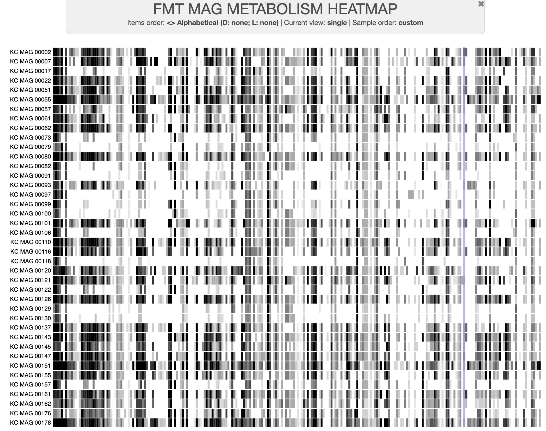
The first iteration of our metabolism heatmap, without an informative organization of the data.
To organize the data nicely, we can cluster the data in each dimension and add the resulting dendrograms to the interface. To do that, we need to go back to the command line. Before you exit the interface, save your settings by clicking the ‘Save State’ button at the bottom of the ‘Main’ settings panel, and save it as the state called ‘default’ so that the interface automatically loads these settings the next time you open this heatmap. Then you can go back to the terminal and hit Ctrl-C to get your prompt back.
First, we will cluster the pathways so that metabolisms with similar distributions across MAGs will be closer together. That will organize the columns of the heatmap (‘items’) in the interface. We can do this clustering directly with the same matrix file that we gave to anvi-interactive earlier, using the program anvi-matrix-to-newick:
anvi-matrix-to-newick FMT_MAG_metabolism-module_pathwise_completeness-MATRIX.txt -o module_organization.newick
Now we want to cluster the genomes according to their metabolic capacity, so that MAGs with similar capacities will be closer together (organizing the rows of the heatmap, aka ‘layers’, in the interface). Since anvi-matrix-to-newick clusters the elements in the rows of the input matrix (which are metabolic modules), we first need to transpose the matrix to have the genomes in the rows instead. Luckily, anvi’o has a convenient little script for that, too.
anvi-script-transpose-matrix FMT_MAG_metabolism-module_pathwise_completeness-MATRIX.txt \
          -o FMT_MAG_metabolism-module_pathwise_completeness-MATRIX-TRANSPOSED.txt
anvi-matrix-to-newick FMT_MAG_metabolism-module_pathwise_completeness-MATRIX-TRANSPOSED.txt -o mag_organization.newick
Now we have two dendrograms, one for each side of the heatmap. Let’s add them to the display by importing them into the profile database. In anvi’o interface lingo, the module dendrogram will be an ‘item order’, and the MAG dendrogram will be a ‘layer order’. Item orders can be provided directly to anvi-interactive using the -t flag, or imported via anvi-import-items-order. We will do the latter.
anvi-import-items-order -i module_organization.newick \
                        -p modules_heatmap.db \
                        --name module_organization
Layer orders have to be imported into the database using anvi-import-misc-data, which requires copying the tree into a tab-delimited file that also describes the name and type of the ordering. We will create this file quickly on the command line, but you can see more information in this tutorial.
TREE=$(cat mag_organization.newick)  # copy the dendrogram into a variable called 'TREE'
echo -e "item_name\tdata_type\tdata_value\nmag_organization\tnewick\t$TREE" > layer_order.txt # put it into a file
# import into the database
anvi-import-misc-data -p modules_heatmap.db \
                      -t layer_orders \
                      layer_order.txt
Then we can re-run the interactive interface. Here is the command again:
anvi-interactive -d FMT_MAG_metabolism-module_pathwise_completeness-MATRIX.txt \
                 -p modules_heatmap.db \
                 --manual \
                 --title "FMT MAG METABOLISM HEATMAP"
This time, open the ‘Main’ settings panel and change the ‘Items order’ to be ‘Module organization’. Then, switch to the ‘Layers’ panel and change the ‘Order by’ setting to ‘mag_organization (tree)`. After you click ‘Draw’, the heatmap will show some nice patterns.
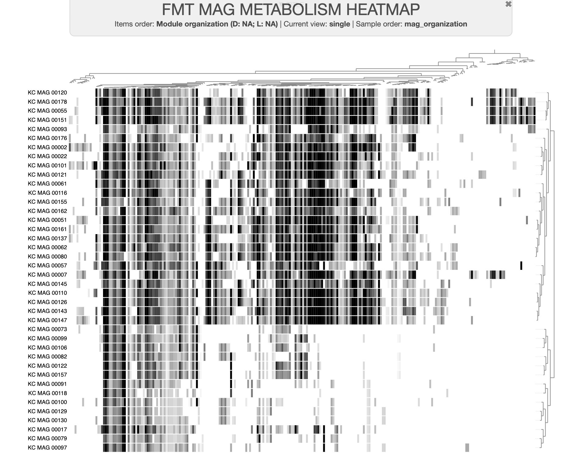
The second iteration of our metabolism heatmap, nicely organized now.
It looks much better now, but one more thing is missing from the display. We don’t know which MAG belongs to which group. We should add their labels. Save the state again (you can overwrite the ‘default’ state), and go back to the terminal. We will import the MAG group as additional data for layers, using the MAG_groups.txt file that already exists in the datapack, like this:
anvi-import-misc-data -p modules_heatmap.db \
                      -t layers \
                      MAG_groups.txt
Then, you can open the interface again (use the same command), and you should see the MAG groups on the side of the heatmap. Here is how it looks (with the ‘low-fitness’ and ‘high-fitness’ groups colored in red and blue, respectively):
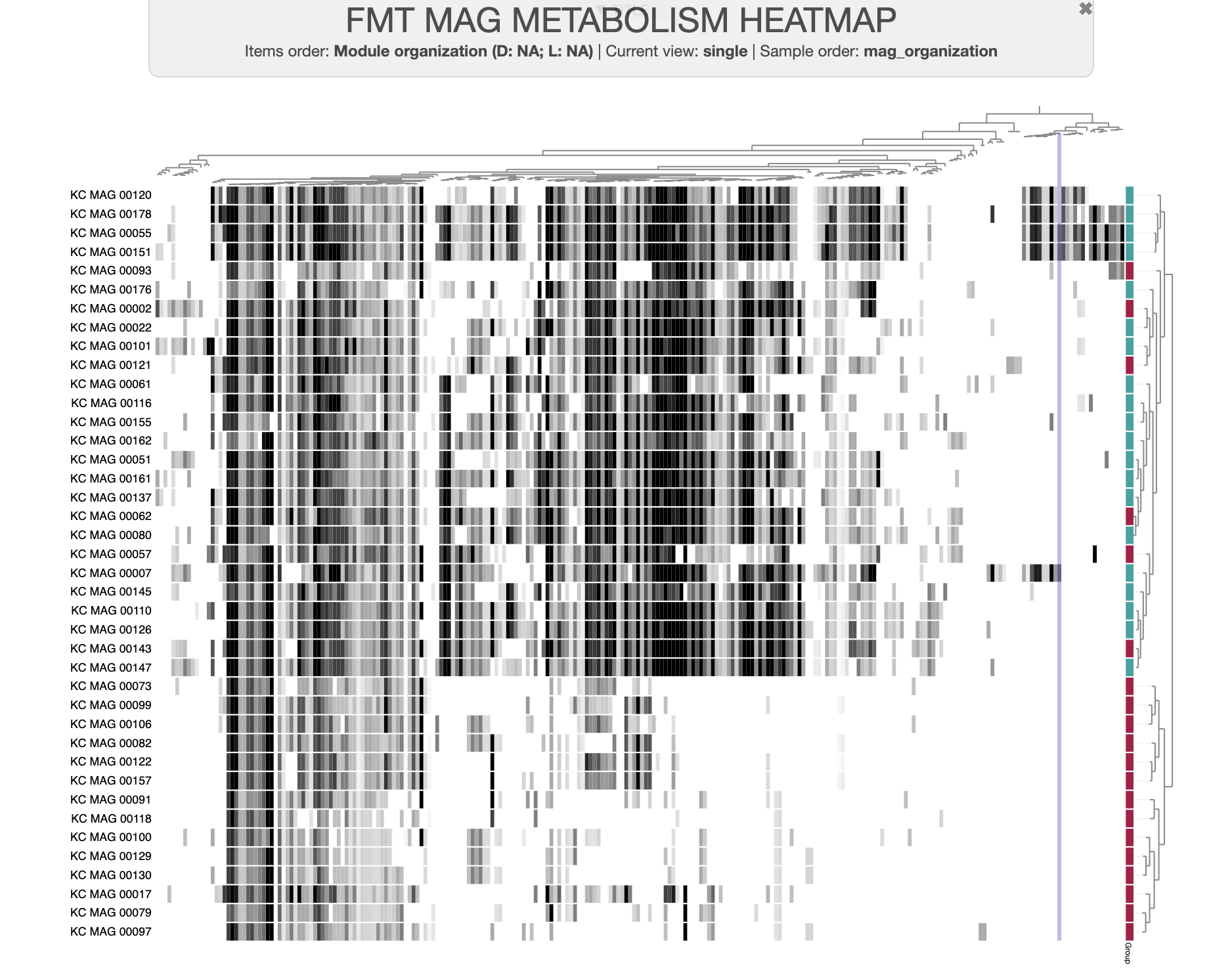
The final iteration of our metabolism heatmap, with colored groups.
In this final heatmap, we can nicely see the pattern that some MAGs are missing many metabolic pathways compared to other MAGs. You can open the ‘Mouse’ panel on the right side of the screen and hover over the heatmap to find out the names of the pathways that are differentially distributed between the groups. But it might still be difficult to tell which specific pathways best distinguish between the two groups. For that task, we need the help of a statistical test.
Finding enriched metabolic pathways
Anvi’o has a program for computing enrichment of metabolic modules in different groups of genomes, and that program is anvi-compute-metabolic-enrichment. It will compute an enrichment score and a list of associated groups for each module that is present in at least one genome (modules are considered ‘present’ in a genome if they have a high enough completeness score in that genome, based upon the threshold we discussed earlier).
To run this program, you must provide it with the modules mode output file we generated in the last section, as well as a groups-txt file that matches each genome to its group name. The latter file is provided in the datapack, so you don’t need to generate it yourself. Here is the code to run the enrichment program:
anvi-compute-metabolic-enrichment -M FMT_MAG_metabolism_modules.txt \
                                  -G MAG_groups.txt \
                                  -o metabolic-enrichment.txt
The result will be a functional-enrichment-txt file describing the name, enrichment score, associated groups, and other information about each metabolic module.
Here are the first 10 lines of this file (scroll to the right to see more columns):
| MODULE | enrichment_score | unadjusted_p_value | adjusted_q_value | associated_groups | accession | sample_ids | p_LOW_FITNESS | N_LOW_FITNESS | p_HIG_FITNESS | N_HIG_FITNESS |
|---|---|---|---|---|---|---|---|---|---|---|
| Isoleucine biosynthesis, threonine => 2-oxobutanoate => isoleucine | 22.556406615904546 | 2.040628701217595e-6 | 5.9487214399712077e-5 | HIG_FITNESS | M00570 | KC_MAG_00002,KC_MAG_00007,KC_MAG_00022,KC_MAG_00051,KC_MAG_00055,KC_MAG_00061,KC_MAG_00062,KC_MAG_00080,KC_MAG_00101,KC_MAG_00110,KC_MAG_00120,KC_MAG_00126,KC_MAG_00137,KC_MAG_00143,KC_MAG_00145,KC_MAG_00147,KC_MAG_00151,KC_MAG_00155,KC_MAG_00161,KC_MAG_00176,KC_MAG_00178 | 0.15 | 20 | 0.9 | 20 |
| Valine/isoleucine biosynthesis, pyruvate => valine / 2-oxobutanoate => isoleucine | 22.556406615904546 | 2.040628701217595e-6 | 5.9487214399712077e-5 | HIG_FITNESS | M00019 | KC_MAG_00002,KC_MAG_00007,KC_MAG_00022,KC_MAG_00051,KC_MAG_00055,KC_MAG_00061,KC_MAG_00062,KC_MAG_00080,KC_MAG_00101,KC_MAG_00110,KC_MAG_00120,KC_MAG_00126,KC_MAG_00137,KC_MAG_00143,KC_MAG_00145,KC_MAG_00147,KC_MAG_00151,KC_MAG_00155,KC_MAG_00161,KC_MAG_00176,KC_MAG_00178 | 0.15 | 20 | 0.9 | 20 |
| C5 isoprenoid biosynthesis, non-mevalonate pathway | 19.26014349752904 | 1.1406274710490811e-5 | 1.8720515628368965e-4 | HIG_FITNESS | M00096 | KC_MAG_00002,KC_MAG_00007,KC_MAG_00017,KC_MAG_00022,KC_MAG_00051,KC_MAG_00055,KC_MAG_00057,KC_MAG_00061,KC_MAG_00062,KC_MAG_00080,KC_MAG_00093,KC_MAG_00101,KC_MAG_00110,KC_MAG_00116,KC_MAG_00120,KC_MAG_00121,KC_MAG_00126,KC_MAG_00137,KC_MAG_00143,KC_MAG_00145,KC_MAG_00147,KC_MAG_00151,KC_MAG_00155,KC_MAG_00161,KC_MAG_00162,KC_MAG_00176,KC_MAG_00178 | 0.35 | 20 | 1 | 20 |
| De novo purine biosynthesis, PRPP + glutamine => IMP | 18.026729736369713 | 2.1782491508385217e-5 | 1.8720515628368965e-4 | HIG_FITNESS | M00048 | KC_MAG_00002,KC_MAG_00007,KC_MAG_00022,KC_MAG_00051,KC_MAG_00055,KC_MAG_00057,KC_MAG_00061,KC_MAG_00062,KC_MAG_00080,KC_MAG_00093,KC_MAG_00101,KC_MAG_00110,KC_MAG_00116,KC_MAG_00120,KC_MAG_00121,KC_MAG_00126,KC_MAG_00137,KC_MAG_00143,KC_MAG_00147,KC_MAG_00151,KC_MAG_00155,KC_MAG_00161,KC_MAG_00162,KC_MAG_00176,KC_MAG_00178 | 0.3 | 20 | 0.95 | 20 |
| Lysine biosynthesis, DAP dehydrogenase pathway, aspartate => lysine | 18.026729736369713 | 2.1782491508385217e-5 | 1.8720515628368965e-4 | HIG_FITNESS | M00526 | KC_MAG_00002,KC_MAG_00007,KC_MAG_00022,KC_MAG_00051,KC_MAG_00055,KC_MAG_00057,KC_MAG_00061,KC_MAG_00062,KC_MAG_00080,KC_MAG_00093,KC_MAG_00101,KC_MAG_00110,KC_MAG_00116,KC_MAG_00120,KC_MAG_00121,KC_MAG_00126,KC_MAG_00137,KC_MAG_00143,KC_MAG_00145,KC_MAG_00147,KC_MAG_00151,KC_MAG_00155,KC_MAG_00161,KC_MAG_00176,KC_MAG_00178 | 0.3 | 20 | 0.95 | 20 |
| F-type ATPase, prokaryotes and chloroplasts | 17.289003389888016 | 3.210393689132412e-5 | 1.8720515628368965e-4 | HIG_FITNESS | M00157 | KC_MAG_00007,KC_MAG_00017,KC_MAG_00022,KC_MAG_00051,KC_MAG_00055,KC_MAG_00057,KC_MAG_00061,KC_MAG_00062,KC_MAG_00080,KC_MAG_00093,KC_MAG_00110,KC_MAG_00116,KC_MAG_00120,KC_MAG_00126,KC_MAG_00137,KC_MAG_00143,KC_MAG_00145,KC_MAG_00147,KC_MAG_00151,KC_MAG_00155,KC_MAG_00161,KC_MAG_00176,KC_MAG_00178 | 0.25 | 20 | 0.9 | 20 |
| Histidine biosynthesis, PRPP => histidine | 17.289003389888016 | 3.210393689132412e-5 | 1.8720515628368965e-4 | HIG_FITNESS | M00026 | KC_MAG_00002,KC_MAG_00007,KC_MAG_00022,KC_MAG_00051,KC_MAG_00061,KC_MAG_00062,KC_MAG_00080,KC_MAG_00093,KC_MAG_00101,KC_MAG_00110,KC_MAG_00116,KC_MAG_00120,KC_MAG_00121,KC_MAG_00126,KC_MAG_00137,KC_MAG_00143,KC_MAG_00147,KC_MAG_00151,KC_MAG_00155,KC_MAG_00161,KC_MAG_00162,KC_MAG_00176,KC_MAG_00178 | 0.25 | 20 | 0.9 | 20 |
| Threonine biosynthesis, aspartate => homoserine => threonine | 17.289003389888016 | 3.210393689132412e-5 | 1.8720515628368965e-4 | HIG_FITNESS | M00018 | KC_MAG_00002,KC_MAG_00007,KC_MAG_00022,KC_MAG_00051,KC_MAG_00055,KC_MAG_00061,KC_MAG_00062,KC_MAG_00080,KC_MAG_00093,KC_MAG_00101,KC_MAG_00110,KC_MAG_00116,KC_MAG_00121,KC_MAG_00126,KC_MAG_00137,KC_MAG_00143,KC_MAG_00145,KC_MAG_00147,KC_MAG_00151,KC_MAG_00155,KC_MAG_00161,KC_MAG_00162,KC_MAG_00178 | 0.25 | 20 | 0.9 | 20 |
| Cobalamin biosynthesis, cobyrinate a,c-diamide => cobalamin | 16.942416859777467 | 3.853092320257694e-5 | 1.8720515628368965e-4 | HIG_FITNESS | M00122 | KC_MAG_00007,KC_MAG_00051,KC_MAG_00055,KC_MAG_00057,KC_MAG_00061,KC_MAG_00062,KC_MAG_00080,KC_MAG_00110,KC_MAG_00116,KC_MAG_00126,KC_MAG_00137,KC_MAG_00143,KC_MAG_00145,KC_MAG_00147,KC_MAG_00151,KC_MAG_00155,KC_MAG_00161,KC_MAG_00162,KC_MAG_00178 | 0.15 | 20 | 0.8 | 20 |
Show/Hide Code for getting Table 11
The previous command generates the enrichment output, so all we need to do is convert it to markdown:
head -n 10 metabolic-enrichment.txt | anvi-script-as-markdown
The modules are organized so that those with higher enrichment scores (and lower significance values) are at the top. You can filter the output using the unadjusted_p_value or adjusted_q_value columns to make sure you only keep the modules that are most enriched in one group or another (the adjusted_q_value column is arguably the best one to filter with as this significance value is adjusted for multiple hypothesis testing). For example, in our study we considered any metabolic module with a q-value less than 0.05 to be enriched in its associated group, as long as it was also at least 75% complete in at least 50% of the group members.
The modules in the partial output above represent the metabolic pathways with the highest enrichment scores in our MAGs. All of the modules shown passed our filtering criteria - they have q-values less than 0.05 and are present in at least 10/20 of their associated group. In total, our group found 33 different KEGG modules that were enriched in these MAGs, including the above 9. You can find out which modules these are by taking a look at our supplementary table 7, sheet (d).
You will see that all 9 of the above modules are enriched in the “high-fitness” group of MAGs - and indeed, all 33 modules that passed our filters were enriched in this group. You might also notice that most of the enriched modules are biosynthesis pathways, particularly of amino acids and essential cofactors. As we discuss in the paper, this indicated to us that “high-fitness” populations were successful in colonizing the FMT recipients because they were metabolically independent - that is, they were able to individually produce the molecules they needed to survive and grow, and thus had a competitive advantage compared to the “low-fitness” populations, which generally did not have these biosynthesis capabilities.
This metabolism estimation and enrichment analysis allowed us to form a clear hypothesis as to why some microbial populations were able to colonize FMT recipients while others weren’t. For a much more robust discussion of the analysis and our conclusions, please read our study.
For some additional metagenome-level analyses that we were not able to perform at the time of the study (since they weren’t fully implemented yet), check out the remaining two sections of the tutorial.
Estimating pathway copy number in a metagenome assembly
This section requires a lot of disk space, computer processing power, and time. If you want to run it yourself, it may be better to do so on a high-performance computer cluster (if you have access to one). But if you are just working on a personal laptop, you might consider simply reading through this section to learn the process and outcome rather than running everything yourself.
Earlier in this tutorial, we learned that pathway copy number could be a relevant metric for unbinned metagenomes. Let’s see this in action, using the metagenomes from the FMT study. You can download a contigs database containing these data using the following commands (it will take some time, and the final uncompressed data will take up ~7.8 GB on your computer).
curl -L https://cloud.uol.de/public.php/dav/files/qbyrxFeapgkiYMT \
     -o FMT_DONOR_A_AND_RECIPIENTS.tar.gz
tar -xvf FMT_DONOR_A_AND_RECIPIENTS.tar.gz && cd FMT_DONOR_A_AND_RECIPIENTS/
rm ../FMT_DONOR_A_AND_RECIPIENTS.tar.gz  # save some space by deleting the archive
anvi-migrate --migrate-quickly *.db  # update the databases to newer versions
The resulting contigs database contains our co-assembly of all metagenomes taken from one FMT donor (Donor A). Since this assembly was previously annotated with an earlier version of KEGG, we have to re-run the annotation with our current snapshot of KEGG. We use the flag --just-do-it to overwrite the existing annotations in the database:
anvi-run-kegg-kofams -c CONTIGS.db \
                     --just-do-it
It will take a long time, because there are 698,938 gene calls in this database that all have to be checked against the 24,217 KOfam profiles in the KEGG database. It took about 3 hours on our HPC with --num-threads 40.
When this is finished, you can estimate pathway copy numbers in this assembly like so:
anvi-estimate-metabolism -c CONTIGS.db \
                         -O DONOR_A \
                         --output-modes modules \
                         --add-copy-number
You will notice in the program output that lots of modules are considered ‘complete’ in this assembly, which makes sense because we have combined the KOfam annotations from all organisms represented across all the metagenomes:
Number of complete modules (pathwise) ........: 187
Number of complete modules (stepwise) ........: 180
Clearly, the completeness metric isn’t very useful in this case. What we want to see instead is the copy number of each pathway. Here is a table extracted from the DONOR_A_modules.txt output file, showing the copy numbers for the first 10 modules:
| module | module_name | pathwise_copy_number | stepwise_copy_number | per_step_copy_numbers |
|---|---|---|---|---|
| M00001 | Glycolysis (Embden-Meyerhof pathway), glucose => pyruvate | 211 | 186 | 319,237,459,437,259,186,351,291,263 |
| M00002 | Glycolysis, core module involving three-carbon compounds | 209 | 186 | 259,186,351,291,263 |
| M00003 | Gluconeogenesis, oxaloacetate => fructose-6P | 185 | 138 | 169,291,351,209,186,259,138 |
| M00307 | Pyruvate oxidation, pyruvate => acetyl-CoA | 244 | 286 | 286 |
| M00009 | Citrate cycle (TCA cycle, Krebs cycle) | 20 | 8 | 244,8,180,74,25,21,182,24 |
| M00010 | Citrate cycle, first carbon oxidation, oxaloacetate => 2-oxoglutarate | 7 | 8 | 244,8,180 |
| M00011 | Citrate cycle, second carbon oxidation, 2-oxoglutarate => oxaloacetate | 20 | 21 | 74,25,21,182,24 |
| M00004 | Pentose phosphate pathway (Pentose phosphate cycle) | 119 | 26 | 26,49,227,289,501,148 |
| M00006 | Pentose phosphate pathway, oxidative phase, glucose 6P => ribulose 5P | 26 | 26 | 26,49 |
| M00007 | Pentose phosphate pathway, non-oxidative phase, fructose 6P => ribose 5P | 227 | 148 | 501,148,227,289 |
Show/Hide Code for getting Table 12
First we extract only the columns containing the module name and copy number information:
cut -f 1,3,18- DONOR_A_modules.txt > table_12.txt
Then we convert it to markdown:
head -n 11 table_12.txt | anvi-script-as-markdown
The pathwise metric gives us the maximum copy number of the most complete paths through the module, and those ‘most complete paths’ may not represent the path used by all of the organisms in the metagenome. That means that, in practice, pathwise copy number is not usually as useful for analyzing metagenomes as stepwise copy number. Stepwise copy number accounts for all possible variations of a given pathway and reports the minimum copy number across all steps – we should focus on this metric when analyzing the metagenome assembly.
But first, so we can better understand how many microbial populations are contributing to these metrics, let’s estimate the number of microbes described in the co-assembly. Here is a quick little Python script to do this, using the NumGenomesEstimator class in anvi’o. To run these commands, type python in your terminal to open the Python interpreter, then copy and paste each command below:
import anvio
from anvio.hmmops import NumGenomesEstimator
estimates = NumGenomesEstimator("CONTIGS.db").estimates_dict
estimates # show the full data structure containing the estimated number of populations
print(estimates['Bacteria_71']['num_genomes']) # specifically print the number of bacteria estimated
print(estimates['Campbell_et_al']['num_genomes']) # (using two different SCG collections)
exit() # leave the Python interpreter
The NumGenomesEstimator class estimates the number of populations in the assembly by calculating the mode of the number of single-copy core gene annotations. You will see in the output that 1) the estimates depend on which (domain-specific) collection of single-copy core genes is used, 2) that no archeael or protist populations are present in the assembly, and 3) there are approximately 179-184 bacteria in this co-assembly from Donor A. When you look at the table above, you can see several pathways with a stepwise copy number which is about the same as the number of bacteria in the assembly – for instance, the various parts of glycolysis, and the non-oxidative phase of the pentose phosphate pathway. Those are fairly common pathways and it makes sense to assume that each microbial population we found in the donor’s stool has those capacity. Some pathways are present in more copies than we have bacteria, which could mean that some populations harbor multiple versions of the pathway (or multiple copies of the same enzymes). This is more likely to happen with pathways that utilize multi-purpose enzymes that can be used for other purposes in the cell.
Earlier, we saw that some of our MAGs (the ‘high-fitness’ ones) had a lot of biosynthetic capabilities while the ‘low-fitness’ group did not. This metagenome assembly (which was generated from FMT donor metagenomes) should include a combination of high- and low-fitness MAGs, so if we look at the biosynthesis pathways enriched in the high-fitness group we should see that there are fewer copies of these pathways than there are bacteria. You can run the following commands to search for some of the enriched pathways and see their stepwise copy numbers. The module numbers were taken from the enrichment output we saw in the previous section.
head -n 1 DONOR_A_modules.txt | cut -f 1,3,19 > table_13.txt
for m in M00570 M00019 M00096 M00048 M00526 M00026 M00018 M00122; do \
  grep -e "^$m" DONOR_A_modules.txt | cut -f 1,3,19 >> table_13.txt; \
done
Here is what the resulting table looks like:
| module | module_name | stepwise_copy_number |
|---|---|---|
| M00570 | Isoleucine biosynthesis, threonine => 2-oxobutanoate => isoleucine | 172 |
| M00019 | Valine/isoleucine biosynthesis, pyruvate => valine / 2-oxobutanoate => isoleucine | 172 |
| M00096 | C5 isoprenoid biosynthesis, non-mevalonate pathway | 135 |
| M00048 | De novo purine biosynthesis, PRPP + glutamine => IMP | 149 |
| M00526 | Lysine biosynthesis, DAP dehydrogenase pathway, aspartate => lysine | 96 |
| M00026 | Histidine biosynthesis, PRPP => histidine | 124 |
| M00018 | Threonine biosynthesis, aspartate => homoserine => threonine | 134 |
| M00122 | Cobalamin biosynthesis, cobyrinate a,c-diamide => cobalamin | 123 |
Show/Hide Code for getting Table 13
We already generated the table above, so here we just convert it to markdown:
cat table_13.txt | anvi-script-as-markdown
And indeed, for most of these, their stepwise copy number is below the number of bacterial populations (n = ~179-184) predicted to be in the assembly, as expected.
Exploring pathway coverage in metagenomes
The contigs database that we were working with above came with an associated profile database that contains the read recruitment data from several metagenomes, sampled in time-series (before and after the FMT) from stool Donor A and their stool recipients. Let’s use this information to look at the coverage of pathways over time.
We can include pathway-specific gene coverage information in the output from anvi-estimate-metabolism by adding the --add-coverage flag and the path to the profile database in the command (this time, we didn’t bother adding copy numbers since we will only be looking at the coverage columns in the output):
rm DONOR_A_modules.txt # we will regenerate this output file
anvi-estimate-metabolism -c CONTIGS.db \
                         -O DONOR_A \
                         --output-modes modules \
                         --add-coverage \
                         -p PROFILE.db
The command will take much longer to run this time, because anvi’o will compute the gene coverage values on the fly (and since there are so many metagenomes in this database, it requires a LOT of memory. We ran it on our HPC with 1.5Tb of memory, and it still took about an hour). The resulting output file will contain several additional columns per metagenome containing 1) the coverage/detection of each gene in the pathway within that metagenome and 2) the average coverage of all genes in the pathway within that metagenome, as described in this documentation page. Since that is a lot of output to go through, let’s simplify by picking a few samples from one FMT recipient and looking only at the average coverage columns.
We’ll check the time-series for recipient number 2, who was sampled twice pre-FMT and 5 times post-FMT. The following commands will generate a table containing the average coverage of pathways, across this time-series of 7 metagenomes sampled from recipient 2 before and after FMT:
# first we determine which columns we need
head -n 1 DONOR_A_modules.txt | tr '\t' '\n' | nl | grep "DA_R02_CDI" | grep "avg_coverage"

# extract those columns, plus the module ID and name
cut -f 1,3,79,81,83,85,87,89,91 DONOR_A_modules.txt > DA_R02_CDI.txt
If we extract the entries for the enriched biosynthesis pathways that we looked at before, you will see the following:
| module | module_name | DA_R02_CDI_C_01_PRE_avg_coverage | DA_R02_CDI_C_02_PRE_avg_coverage | DA_R02_CDI_C_03_POST_avg_coverage | DA_R02_CDI_C_04_POST_avg_coverage | DA_R02_CDI_C_05_POST_avg_coverage | DA_R02_CDI_C_06_POST_avg_coverage | DA_R02_CDI_C_07_POST_avg_coverage |
|---|---|---|---|---|---|---|---|---|
| M00570 | Isoleucine biosynthesis, threonine => 2-oxobutanoate => isoleucine | 7.030147747823216 | 8.127254306220932 | 10.776163879006777 | 9.21669920940846 | 7.38696713268554 | 22.6383919730815 | 9.580871067027301 |
| M00019 | Valine/isoleucine biosynthesis, pyruvate => valine / 2-oxobutanoate => isoleucine | 7.088530679346055 | 8.454480551316102 | 10.999009890609942 | 9.666443811889957 | 7.536697981663868 | 23.200999343921772 | 9.97102520636212 |
| M00096 | C5 isoprenoid biosynthesis, non-mevalonate pathway | 5.432252681706168 | 7.517438843988805 | 10.13562430009517 | 9.335302646837535 | 6.661625080298928 | 20.732497351757356 | 8.965614083024139 |
| M00048 | De novo purine biosynthesis, PRPP + glutamine => IMP | 6.0201337640841235 | 9.00528497504295 | 10.771679712768764 | 9.679545034513543 | 6.7888392240324675 | 21.4037746898059 | 8.899770054197274 |
| M00526 | Lysine biosynthesis, DAP dehydrogenase pathway, aspartate => lysine | 6.50032763273386 | 8.641326627532365 | 10.120097208395494 | 8.850149126608361 | 5.967971953044325 | 18.77991723628484 | 8.441058665334717 |
| M00026 | Histidine biosynthesis, PRPP => histidine | 4.040690209232013 | 5.43125656737785 | 11.062471930041422 | 9.46079543572338 | 6.856359140252714 | 21.615225789671697 | 9.477373554958936 |
| M00018 | Threonine biosynthesis, aspartate => homoserine => threonine | 5.762365477068536 | 7.912415988495419 | 9.497473572196393 | 8.90843963942808 | 5.812884811492004 | 18.514104313872405 | 8.403356560258128 |
| M00122 | Cobalamin biosynthesis, cobyrinate a,c-diamide => cobalamin | 3.8385902188440024 | 6.661775130193691 | 10.353893326696435 | 9.851028260300374 | 6.155289800418834 | 20.55065270641417 | 9.68897061113826 |
Show/Hide Code for getting Table 14
This command extracts the relevant pathways from the table we just generated above:
head -n 1 DA_R02_CDI.txt > table_14.txt
for m in M00570 M00019 M00096 M00048 M00526 M00026 M00018 M00122; do \
  grep -e "^$m" DA_R02_CDI.txt >> table_14.txt; \
done
And we convert that to markdown:
cat table_14.txt | anvi-script-as-markdown
You will see that the average gene coverages in these pathways rise and fall over the course of the time series. They are generally lower in the pre-FMT samples (~3-7x coverage). Post-FMT, the coverages are higher (~9-11x). They dip a bit in the 5th sample but reach a peak in the 6th (~18-23x). If you check the first figure in our paper (which you can also see in this section of our reproducible workflow), you will see that these trends correspond directly to the rise and fall of the sequencing depth of these metagenomes from recipient 2 (see the ‘Total Num Reads’ barplots on the right): the 5th sample has the lowest sequencing depth and the 6th has the highest.
So that all makes sense. If you wanted to analyze the differences in coverage values of these pathways across the time series, you would have to normalize by sequencing depth. But that is a story for another tutorial. :)
Conclusion
We hope the tutorial above helped you to learn how to run metabolism analyses in anvi’o on your own data. If anything was not clear, please feel free to comment below or reach out to us on Discord with questions. Thanks for reading!