Metabin refinement and population genetics using human tongue metagenomes


Table of Contents
Real world datasets are complicated, and it can be difficult to accurately capture this in tutorials due to time and space constraints. The infamous Infant Gut Tutorial covers the basics of both binning and population genetics on an extremely simple dataset, which is great for learning but the process and results are not necessarily representative of what one would actually end up doing/seeing in a large-scale ‘omics study. Take binning, for example – if you have dozens of large co-assemblies in your dataset, you won’t have the time to do manual binning (and even if you wanted to, chances are that your dataset would be too large to visualize in the anvi’o interactive interface). And microbial communities containing hundreds of populations rarely show perfectly clean, easy-to-bin patterns of sequence composition and differential coverage. As for population genetics, our existing tutorial shows you how to do the thing, but leaves out some context for the question and important parameter decisions along the way.
With that in mind, we created this tutorial to show a more realistic example of how to work on both metagenomic binning and population genetics in anvi’o, using real-world data from the human oral microbiome as generated in the paper “Functional and genetic markers of niche partitioning among enigmatic members of the human oral microbiome” by Shaiber et al (2020). Our goal is to show you the following:
- How to run a read recruitment workflow from many samples to a co-assembly, to generate differential coverage data for binning as well as variant data for population genetics
- How to manually refine a ‘metabin’ that was automatically generated by CONCOCT and encompasses several microbial populations into a few smaller yet high-quality bins
- How to set some key parameters in a population genetics analysis that answers a (somewhat) realistic research question
Of course, we are still constrained a little bit by the time and computational resources allowed by a typical tutorial session. We will be working with a smallish co-assembly that is entirely visualizable in the anvi’o interactive interface (unlike many real-world datasets). And it is unlikely that we will actually run the read recruitment workflow in a tutorial setting (but we will give you all the tools to do so in case you want to try it at home).
Without further ado, let’s begin :)
Our dataset and questions
We are taking advantage of the publicly-available data from Shaiber et al 2020. This study described a time-series of tongue and plague metagenomes taken from several human individuals, most of which were paired in male-female couples. This sampling strategy is particularly effective for metagenomic binning for the following reasons. First, having multiple samples from a single individual enabled the authors to do co-assembly, which effectively increases the coverage and likelihood of catching low-abundance populations (at the cost of increasing the overall complexity, which can break assembly algorithms). Second, we know that similar populations likely occur across different individuals and it therefore makes sense to map multiple individuals to a given co-assembly to leverage more differential coverage signals – this was not the strategy used in the Shaiber et al 2020 paper, but it will work quite well for our purposes today.
Here are the questions we want to answer using this dataset:
- What microbial populations can we recover high-quality metagenome-assembled genomes (MAGs) for by refining ‘metabins’?
- Do the individuals in a couple share similar populations in their oral microbiomes? To put it another way – can the population variants specific to a given individual help us distinguish between the couples?
In order to answer these questions at a smaller scale, we will be using a subset of the data from the 2020 study - a co-assembly of 5 tongue samples from the time-series of a single individual (the sample named T-B-M in the original paper), plus 20 tongue metagenomes to recruit reads from. These include the 5 samples used to make the co-assembly and 5 each from three other individuals: T-A-F, T-A-M, and T-B-F.
For the purposes of this tutorial, we will use the co-assembly that was already generated by the study authors. We will start our binning journey from the results of the automatic binning tool CONCOCT (Alneberg et al 2014) that was already run on the co-assembly.
In fact, CONCOCT was run twice – once by specifying -c 10 to force the tool to create exactly 10 ‘metabins’ (each containing multiple microbial populations), and once without enforcing a number of bins (in which case the tool would try to group sequences from exactly one population in each bin). The ‘metabin’ strategy is extremely useful for partitioning your large metagenomic datasets into manageable chunks that can be manually refined, and is described elsewhere in a blog post by Tom and Meren.
The mapping workflow
If all we wanted to do was bin refinement, a read recruitment step wouldn’t really be necessary here. After all, the automatic binning results were already generated using existing read recruitment results whereby the 5 time-series samples were mapped against their co-assembly. So we could have just taken the existing, publicly-available contigs and profile databases from this Figshare and done our bin refinement on that.
But we want more than that. To answer question (2), we also want to see how the tongue-associated populations from the individual T-B-M differ from the tongue-associated populations in the three other individuals (which means we need mapping information from 15 additional samples). And if we are going to map additional samples to the co-assembly anyway, might as well use them to help guide our bin refinement process.
This is probably not a step that you want to run on a laptop. We did it on our high-performance computing cluster (HPC), using the snakemake workflow for metagenomics implemented in anvi-run-workflow. We will show you how we set this workflow up, but there is no need for you to run it yourself - you will be able to download the output of the workflow that is required for the rest of the tutorial in the next section.
Show/Hide You want to run the mapping workflow yourself? Here is how to get the short read data.
To get the metagenome samples, open the SRA Run Selector for the BioProject PRJNA625082 in your favorite web browser. In the filters on the left side, filter for ‘host_tissue_sampled’ = ‘Tongue’ and ‘Assay_Type’ = ‘WGS’ to get all the tongue samples. Then downloaded the metadata table as a CSV. You can then select only the time-series samples from our 4 individuals of interest by running the following code on the metadata table in your terminal:
# keep only accession and sample name
cut -d ',' -f 1,45 Oral_Microbiome_SraRunTable.csv | tr ',' '\t' > oral_samples.txt
# search for sample names of interest and extract to a new file
for n in T_B_M T_B_F T_A_F T_A_M; do \
  grep $n oral_samples.txt >> oral_samps_to_download.txt ; \
done
# extract only the accession for the samples of interest
cut -f 1 oral_samps_to_download.txt > SRA_accession_list.txt
This creates a file of SRA accession numbers that becomes the input to the SRA download workflow. You should put that SRA_accession_list.txt file wherever you want to download those samples (for instance, on your HPC), and then get a default config file for the workflow:
anvi-run-workflow -w sra_download --get-default-config download.json
Feel free to open that config and change the parameters (for instance, number of threads) for each rule according to the computational resources available to you.
When you are ready to download the samples, running the workflow is as simple as this:
anvi-run-workflow -w sra_download -c download.json
If you are running on a cluster, you may want to use the --additional-params (or -A) flag to pass cluster-specific scheduler commands and resource limits to snakemake using flags such as --cluster, --resources, --jobs, etc.
Once the workflow is done, you should have a folder of FASTQ files for 20 metagenome samples. And then you’ll be ready to run the mapping workflow!
So, how did we run the mapping workflow?
First, we got our reference metagenome co-assembly for individual T-B-M by downloading the corresponding contigs and profile database from this Figshare link. Then, we extracted the FASTA file of the contigs, as well as both existing CONCOCT collections that were already stored in the profile database:
# extract le data
tar -xvf T-B-M.tar.gz

# update the dbs to match your current anvi'o version
anvi-migrate --migrate-safe T-B-M/*.db

# get our reference FASTA file
anvi-export-contigs -c T-B-M/CONTIGS.db -o T_B_M-contigs.fa

# export the metabin collection
anvi-export-collection -p T-B-M/PROFILE.db -C CONCOCT_c10 -O CONCOCT_c10

# export the standard CONCOCT collection
anvi-export-collection -p T-B-M/PROFILE.db -C CONCOCT -O CONCOCT
We will use the FASTA file of the co-assembly contigs as the reference in our mapping workflow. The mapping workflow will create a new contigs database out of this FASTA file, and associate the mapping data to that new contigs database via a new (merged) profile database containing the mapping info from all 20 of our samples. Because we’ll get a fresh profile database that won’t have any of the existing collection information in it, we will need to import the collection data (using the collection files we just exported) so that we can do our bin refinement from there. Luckily, because we exported our reference FASTA directly from the contigs database, the split names in the exported collection files will match to the names in the new contigs database. But we are getting ahead of ourselves. First we actually have to run the workflow.
On our HPC, we navigated to the folder where we downloaded the 20 metagenome samples that we want to map against this co-assembly. We created a samples-txt file that describes the paths to each of the samples (you can see the format here). Then we generated a fasta-txt file with the path to our reference co-assembly FASTA, and we got a default config file for the metagenomics workflow:
echo -e "name\tpath\nT_B_M\tT_B_M-contigs.fa" > fasta.txt
anvi-run-workflow -w metagenomics --get-default-config map.json
After modifying the config file a bit to turn on ‘reference mode’, turn off unnecessary rules (like functional annotation),, and increase the number of threads for each rule as much as our cluster could handle, we did a dry run (using the -n dry run flag and -q quiet flag passed directly to snakemake using -A or --additional-params) to see what the workflow would actually run:
anvi-run-workflow -w metagenomics -c map.json -A -n -q
And it showed us the following list of jobs:
job                                  count
---------------------------------  -------
annotate_contigs_database                1
anvi_gen_contigs_database                1
anvi_init_bam                           20
anvi_merge                               1
anvi_profile                            20
anvi_run_hmms                            1
anvi_run_scg_taxonomy                    1
bowtie                                  20
bowtie_build                             1
gen_qc_report                            1
gzip_fastqs                             40
import_percent_of_reads_mapped          20
iu_filter_quality_minoche               20
iu_gen_configs                           1
metagenomics_workflow_target_rule        1
samtools_view                           20
total                                  169
Everything looked okay in the dry run. We have 20 samples, so it makes sense that we are doing all the sample-specific jobs 20 times (the only exception, gzip_fastqs, works individually on R1 and R2 files, so it runs twice per samples).
We very confidently started the workflow using the command:
anvi-run-workflow -w metagenomics -c map.json
And after it finished successfully, we took the resulting contigs database and merged profile database, and we imported the original collections of CONCOCT bins that we extracted previously:
anvi-import-collection -p PROFILE.db -C CONCOCT_c10 CONCOCT_c10.txt -c T_B_M-contigs.db
anvi-import-collection -c T_B_M-contigs.db -p PROFILE.db -C CONCOCT CONCOCT.txt
These are the databases that were put into the datapack for this tutorial, which you can download in the next section.
Refining CONCOCT metabins
First, let’s download the tutorial datapack. Just so you know, the archived databack is about half a gigabyte in size, and once unpacked it will take up ~1.6Gb of space on your computer. If you are okay with that, here are the download commands:
curl -L https://cloud.uol.de/public.php/dav/files/c4TyGoDe3D7XPiq \
     -o BINNING_POPGEN_TUTORIAL.tar.gz
tar -xvf BINNING_POPGEN_TUTORIAL.tar.gz && cd BINNING_POPGEN_TUTORIAL/
You should now be inside the datapack directory on your terminal. The directory should contain 3 databases – the contigs database containing the co-assembly of the 5 time-series tongue metagenomes from one individual (T-B-M), the profile database containing the mapping data from 20 tongue metagenome samples (from the same T-B-M individual as well as three others), and an auxiliary database with lots of extra info related to the mapping (which we will use later).
An initial look at the co-assembly
Let’s take a look at what we have in the database.
anvi-display-contigs-stats T_B_M-contigs.db
A little interactive window should pop up in your browser, filled with useful tables of statistics about the co-assembly. At the top you will see a bar chart of the number of annotations to each single-copy core gene (SCGs; which can be annotated by running anvi-run-hmms) in the assembly contigs. Here is the chart for the Bacteria_71 set of bacterial SCGs:
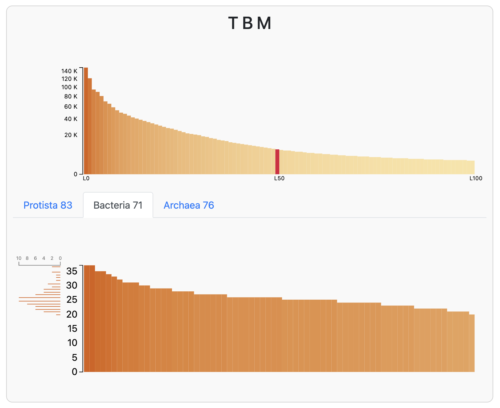
A bar chart of hits to bacterial SCGs in the T-B-M co-assembly
Since we expect that each microbial population should have one copy of each of these SCGs, it looks like we have at least 20 bacterial populations in this co-assmbly (and at most 35). In fact, the most common number of hits to a given bacterial SCG is 25, which is exactly the number of bacterial genomes that anvi’o predicted this assembly to have:
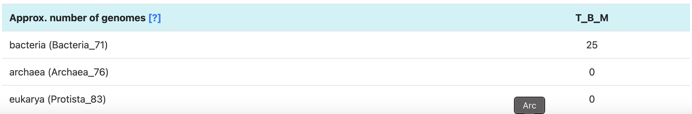
Predicted number of populations in the T-B-M co-assembly, based on SCG counts
If you want to learn more about how anvi’o estimates the number of genomes, you can click the little [?] link in the interactive interface, or just click on this conveniently-placed link to the same documentation.
Anyway, we expect to find at least 25 bacterial populations in this co-assembly (there will probably be even more than that because many of the populations are likely to be incomplete). We’re going to do our best to bin at least some of these populations.
We will be refining metabins that were automatically binned by CONCOCT. Let’s check which collections we have available for this co-assembly. Collections of bins are stored in the profile database, so we pass that database as a parameter to anvi-show-collections-and-bins:
anvi-show-collections-and-bins -p PROFILE.db
You should see two collections. One of them is just called CONCOCT and it contains over 50 bins:
Collection: "CONCOCT"
===============================================
Collection ID ................................: CONCOCT
Number of bins ...............................: 58
Number of splits described ...................: 12,499
Number of contigs described ..................: 12,173
These are the binning results from a standard run of CONCOCT, whereby the program did its best to split each individual microbial population into its own bin. As you can see, the number of bins is much larger than the expected number of microbial populations based on single-copy core genes. It is always possible (and perhaps even likely) that we are missing some SCG annotations due to incomplete coverage of less abundant populations. However, it is also possible (and perhaps even very likely) that CONCOCT fragmented some of these population genomes across multiple bins. Which is one reason that we like to use the metabin approach described in this blog post - if you tell CONCOCT to make just a few bins (much less than the number of expected populations), then it is less likely to split sequences from the same population across different bins.
Happily, the second collection in the profile database, CONCOCT_c10, is the metabin collection. Shaiber et al. created this collection by running CONCOCT with the -c 10 parameter, to request 10 bins:
Collection: "CONCOCT_c10"
===============================================
Collection ID ................................: CONCOCT_c10
Number of bins ...............................: 10
Number of splits described ...................: 12,499
Number of contigs described ..................: 12,173
Bin names ....................................: Bin_1, Bin_10, Bin_2, Bin_3, Bin_4, Bin_5, Bin_6, Bin_7, Bin_8, Bin_9
This is the collection we are going to work on in just a moment.
First, let’s just take a look at the co-assembly and its mapping data.
anvi-interactive -c T_B_M-contigs.db -p PROFILE.db \
    --title "T-B-M co-assembly"
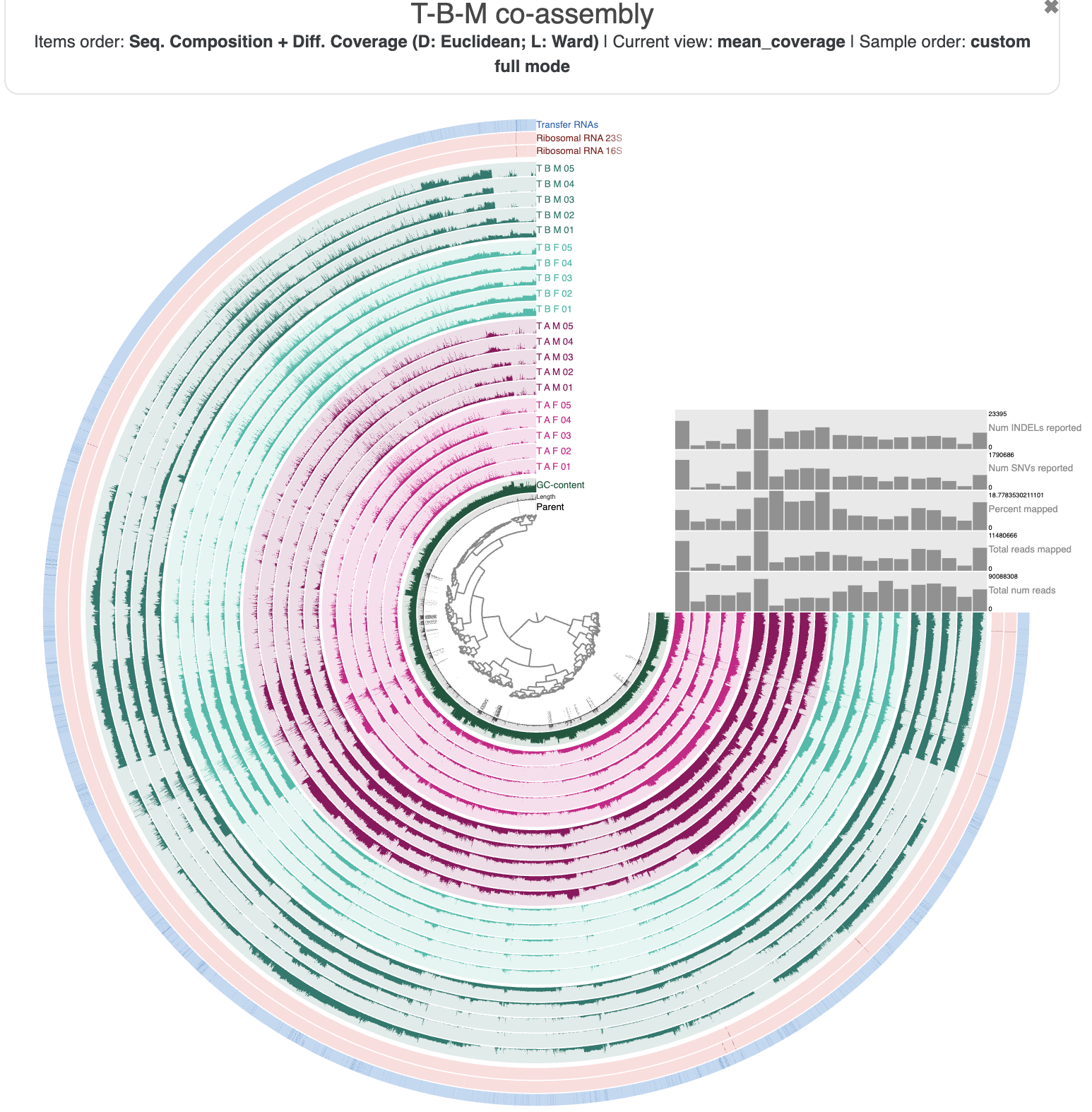
The T-B-M co-assembly in the interactive interface.
The profile database comes with pre-loaded settings to make the visualization a bit more digestible. The sample layers are colored according to which individual they come from - in particular, the 5 T-B-M samples that were used to make the co-assembly are in dark green. We can see coverage patterns in the samples from the other individuals that were mapped to this co-assembly – the other individuals’ tongue microbiomes include similar populations to those in T-B-M’s – which is good news for us because it means we can use the mapping data from the other samples to help guide our bin refinement.
If you check the ‘Items order’ label at the top, you will see that the contigs (technically, their splits) are organized according to their shared sequence composition (tetranucleotide frequency) and differential coverage patterns across all 20 samples. The inner dendrogram displays this organization, and we often use this dendrogram to select which contigs to put into a bin – because we expect that sequences originating from the same genome should have roughly the same composition and follow similar differential coverage patterns.
Just out of curiousity, let’s take a look at how the standard CONCOCT bins group the contigs from the co-assembly. You can either load the bin collection CONCOCT from the ‘Bins’ panel in the interface, or close and re-open the interface with --collection-autoload in the command:
anvi-interactive -c T_B_M-contigs.db -p PROFILE.db \
    --title "T-B-M co-assembly (CONCOCT collection)" \
    --collection-autoload CONCOCT
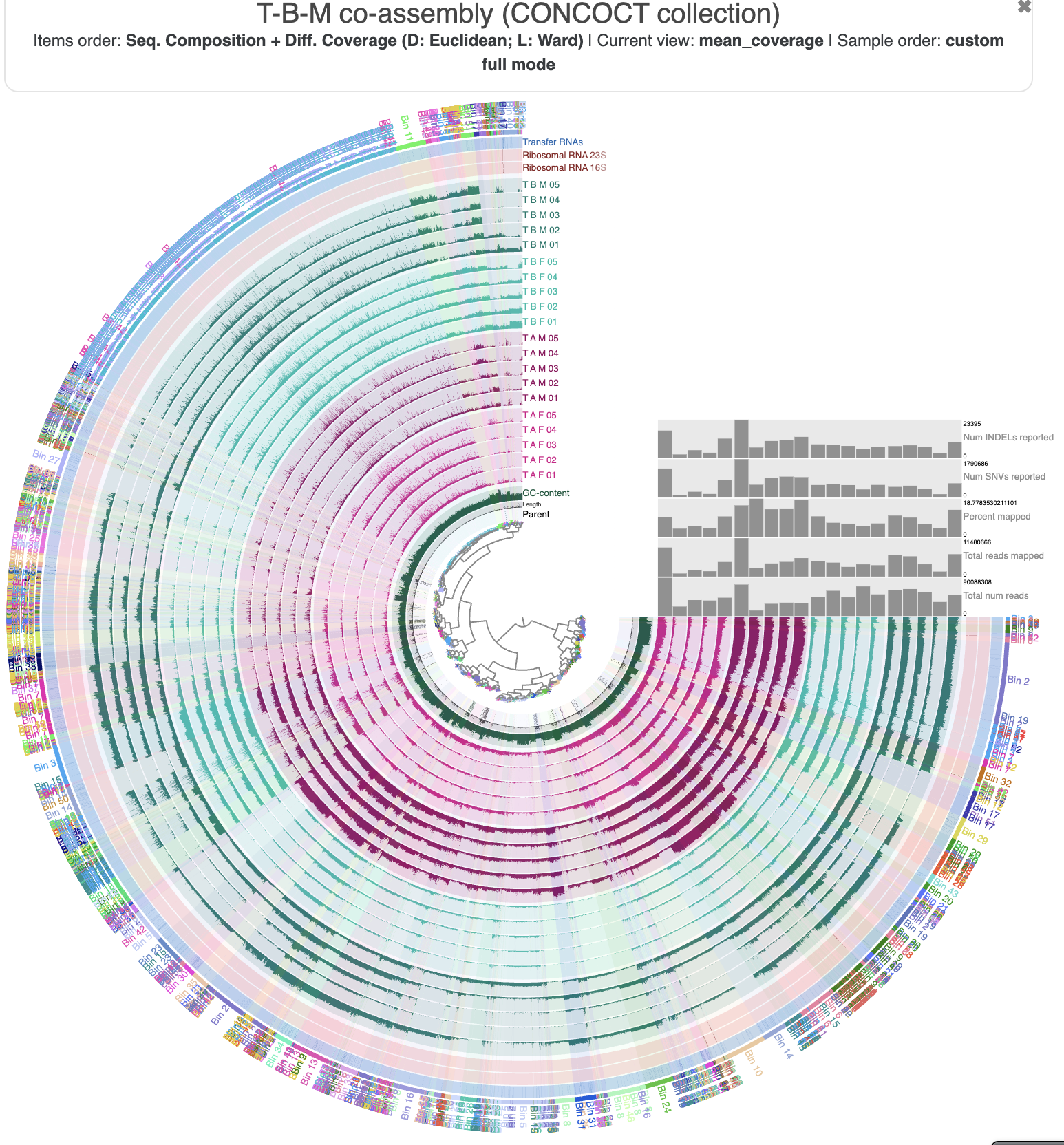
The regular CONCOCT bins
You can see a lot of mixing between the different bins. There are some sections of the figure where a clade on the inner dendrogram has been sorted into a single bin (such as Bin 2, Bin 10, and Bin 11), but for the most part, the bins are quite fragmented. This is exactly what we wanted to avoid by using the metabin technique.
What do the metabins look like? Again, you can load the collection from the interface, or re-start the interface with a new collection name to load:
anvi-interactive -c T_B_M-contigs.db -p PROFILE.db \
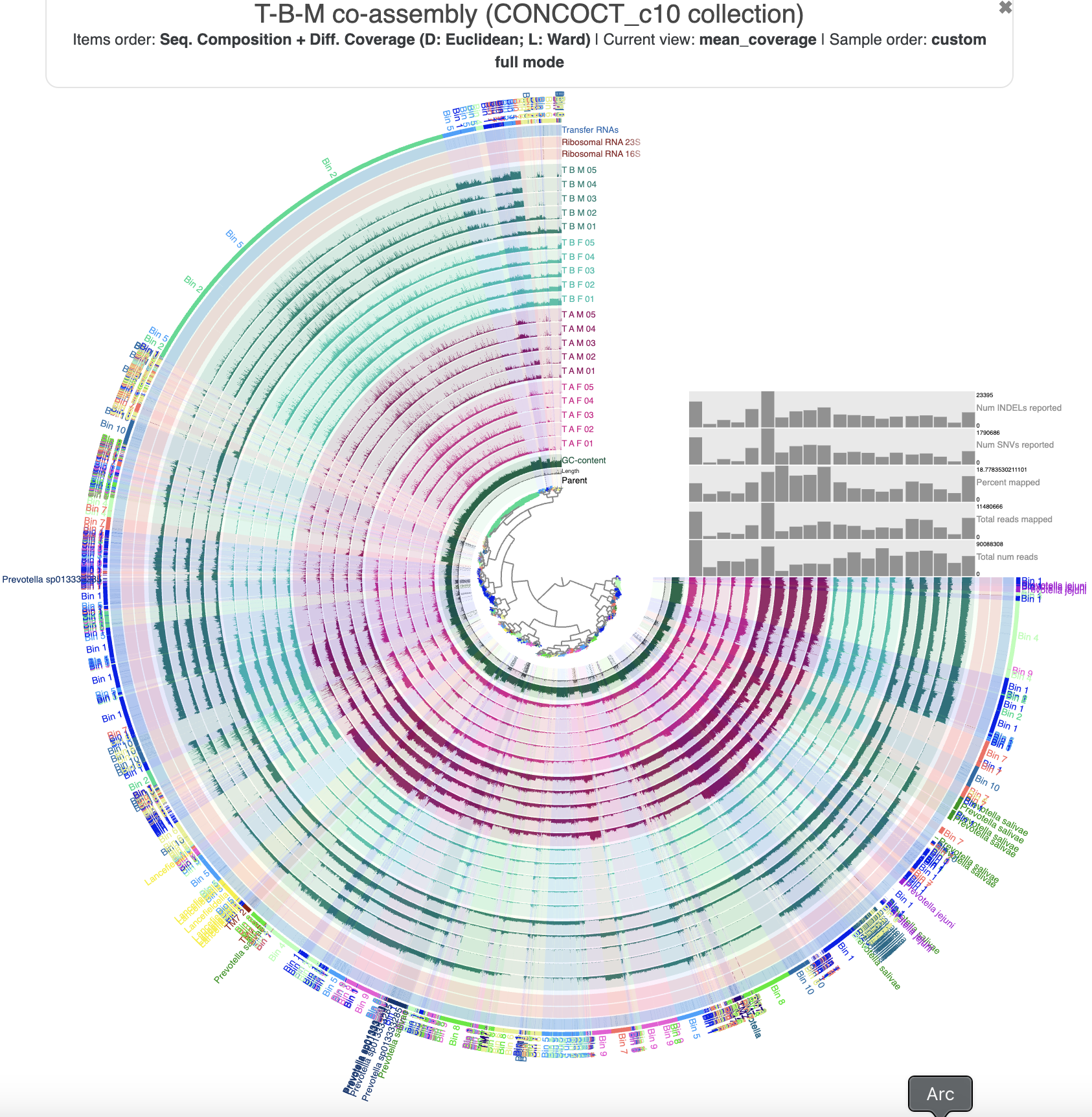
--title "T-B-M co-assembly (CONCOCT_c10 collection)" \
--collection-autoload CONCOCT_c10
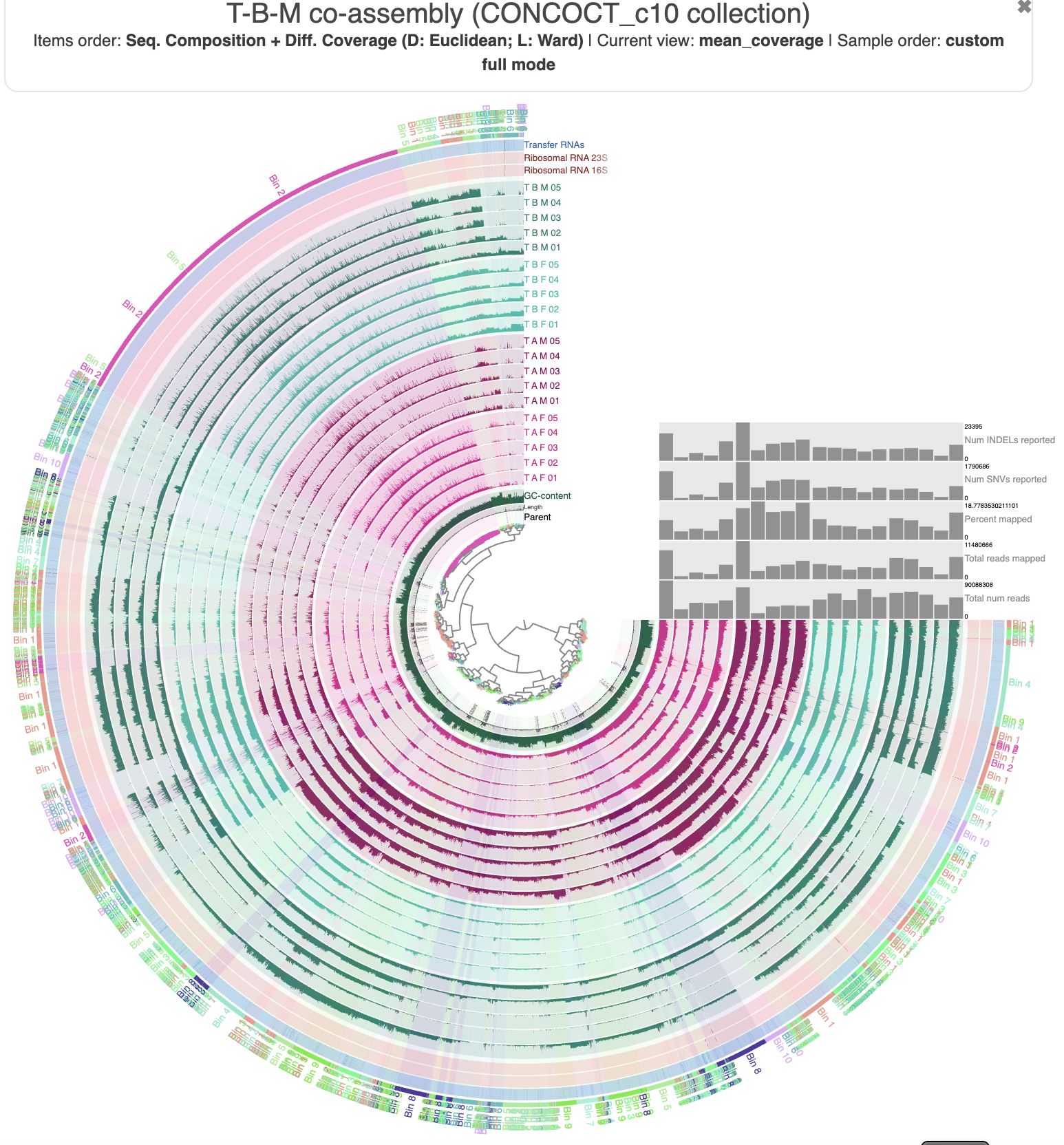
The 10 CONCOCT metabins
It is a little bit better. Now multiple bacterial populations have been purposefully combined into just a few metabins, and we can see a bit less mixing; ie, the binning follows the dendrogram structure better. And in general, the mixing is not as chaotic – many clades of the inner dendrogram are sorted into just two bins. We should be able to work with this output to refine a metabin into some high-quality MAGs.
Why so much mixing? Is CONCOCT doing a really bad job? Maybe. After all, automatic binning of complex metagenomes is an extremely difficult task and algorithmic heuristics won’t always give us an answer we expect. But maybe not. It is important to remember that CONCOCT was given only a fraction of the information shown here to base its binning decisions on. It only used differential coverage signal from the 5 dark green samples from T-B-M – the samples used to make the co-assembly. Here, we are showing mapping information from 15 extra samples from 3 different individuals, and while it seems clear that those individuals harbor similar populations, there is likely still some variation like large-scale insertions and deletions or hyper-variable regions that could confuse the differential coverage signals. So give CONCOCT a break – it is trying its best to live up to our unrealistic expectations. :P
Refining Bin 3
We want to refine a metabin and split it into its component populations. But which metabin should we work on? If you take a look in the ‘Bins’ panel on the interactive interface, you should see the overall completeness and redundancy estimates for each one:
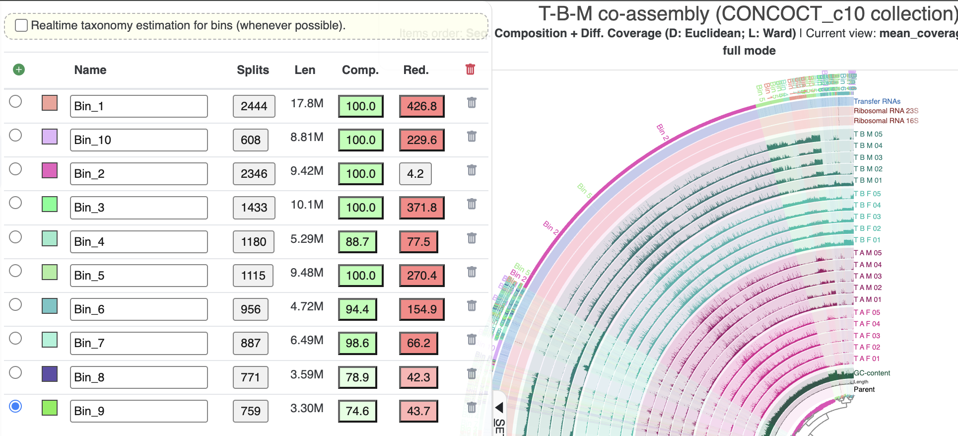
Completion and redundancy of the metabins
As expected, they have a lot of redundancy because each bin contains several microbial populations. The only potential exception is Bin 2, which clearly stands out as one of the only bins that cohesively groups several consecutive clades in the inner dendrogram and seems to represent a single population based on the coverage patterns (though the size of the bin is a bit large for most microbial genomes). So we would like to focus on refining one of the other bins.
Somewhat arbitrarily, we selected the second-largest bin, Bin 3, to refine for this tutorial. Based on its redundancy score, we should be able to obtain at least 4-5 bins out of this metabin (potentially more if the populations are incomplete).
Here is the command to refine Bin 3. It will open the interactive interface again, but this time only showing the contigs (technically, their splits) belonging to Bin 3.
anvi-refine -c T_B_M-contigs.db -p PROFILE.db -C CONCOCT_c10 -b Bin_3
Here is what Bin 3 looks like in the interface:
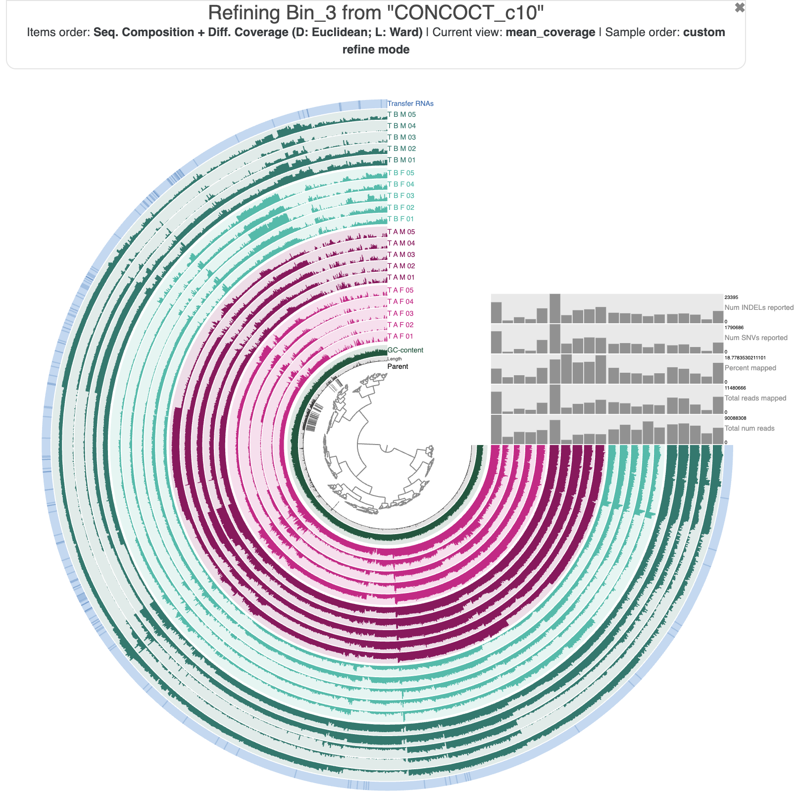
Refining metabin ‘Bin 3’ in the interface’s ‘refine mode’.
Now we can use the dendrogram organization, the differential coverage patterns, and the SCG-based completion/redundancy/taxonomy estimates to identify the subsets of this metabin that represent individual population genomes. Give it a try for yourself, and once you are ready, click the Show/Hide box to see if your results match ours.
Show/Hide Our Bin 3 refinement results.
We focused on the major patterns and ended up with 7 bins in our refined collection. We could have binned much more, but when we tried that, most of the resulting bins were so small/incomplete that they wouldn’t have been useful. Here is what our collection looks like in the ‘refine mode’ interface:
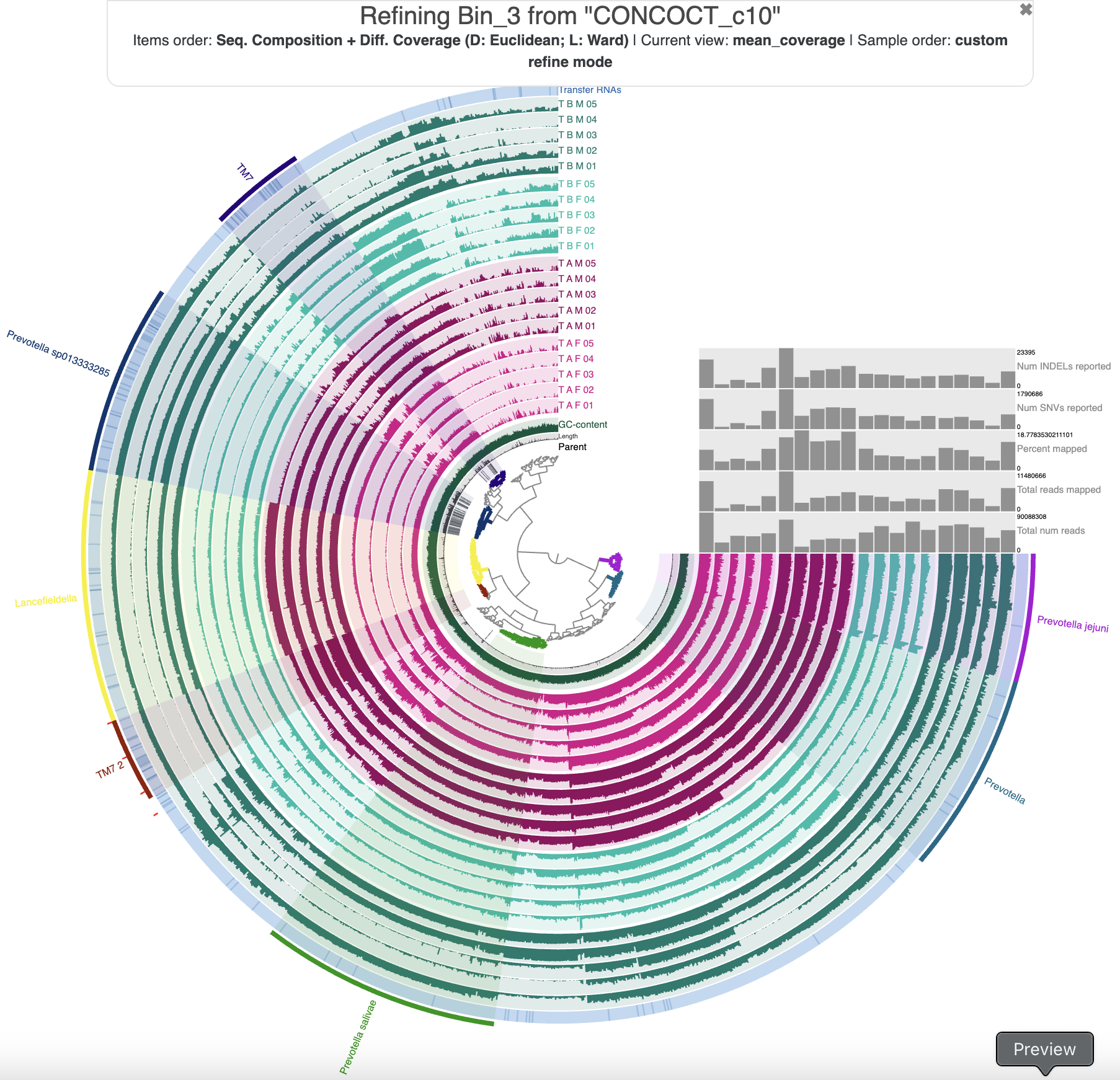
The 7 bins resulting from our refinement.
And here are the bin statistics from the ‘Bins’ panel on the side:
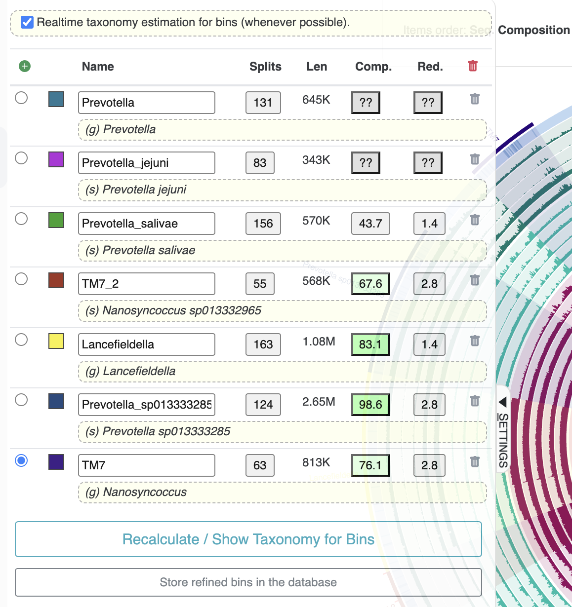
Statistics of the 7 refined bins from metabin ‘Bin 3’.
We named the bins according to the SCG taxonomy estimates. There are several Prevotella populations, but only 1 (Prevotella sp013333285) has a large enough and complete enough bin to be useful. There were also two decent bins for Nanosynococcus species – also known as TM7, these populations were the center of attention in the Shaiber et al. paper, so it is unsurprising that we found them here.
Make sure to hit the button called ‘Store refined bins in database’ in the ‘Bins’ panel to save your work once you are done refining. Please note that this will overwrite your existing larger collection (in our case, this is the CONCOCT_c10 collection), replacing the original metabin (Bin_3) with the set of smaller bins you curated.
Congratulations! You just refined a metabin. :)
If you want to see how your bin looks in the context of the larger co-assembly, you can do that by going back to the regular interactive interface, using the following command to automatically open the (now partially-refined) CONCOCT_c10 collection.
anvi-interactive -c T_B_M-contigs.db -p PROFILE.db \
    --title "T-B-M co-assembly (CONCOCT_c10 collection)" \
    --collection-autoload CONCOCT_c10
Show/Hide Our Bin 3 refinement results, in the co-assembly.
If you want to load our collection of refined bins to view them in the larger context, you can run the following:
anvi-import-collection -p PROFILE.db -C refined_c10 refined.txt -c T_B_M-contigs.db
anvi-import-collection -p PROFILE.db -C refined_Bin_3 refined_Bin_3.txt -c T_B_M-contigs.db
The collection refined_Bin_3 contains only the bins we extracted from the metabin Bin 3, while the collection refined_c10 contains all of those bins in addition to the other metabins (that we didn’t yet refine).
You can then load up the refined_c10 collection like this:
anvi-interactive -c T_B_M-contigs.db -p PROFILE.db \
    --title "T-B-M co-assembly (CONCOCT_c10 collection)" \
    --collection-autoload refined_c10
The updated CONCOCT_c10 collection in the T-B-M co-assembly.
It’s a bit messy, but hopefully you can pick out the locations where Bin 3 turned into all those new refined “sub-bins”. They are dispersed throughout the co-assembly, intermixed with sequences from the other metabins. This shows again that the automatic binning from CONCOCT, even at a coarse ‘metabin’ level, is often at odds with the patterns emerging from the current sequence organization based on tetranucleotide frequency and differential coverage.
It is a bit easier to see how fragmented the new, refined bins are in this organization if we load the refined_Bin_3 collection to see only those 7 bins:
anvi-interactive -c T_B_M-contigs.db -p PROFILE.db \
    --title "T-B-M co-assembly (refined bins collection)" \
    --collection-autoload refined_Bin_3
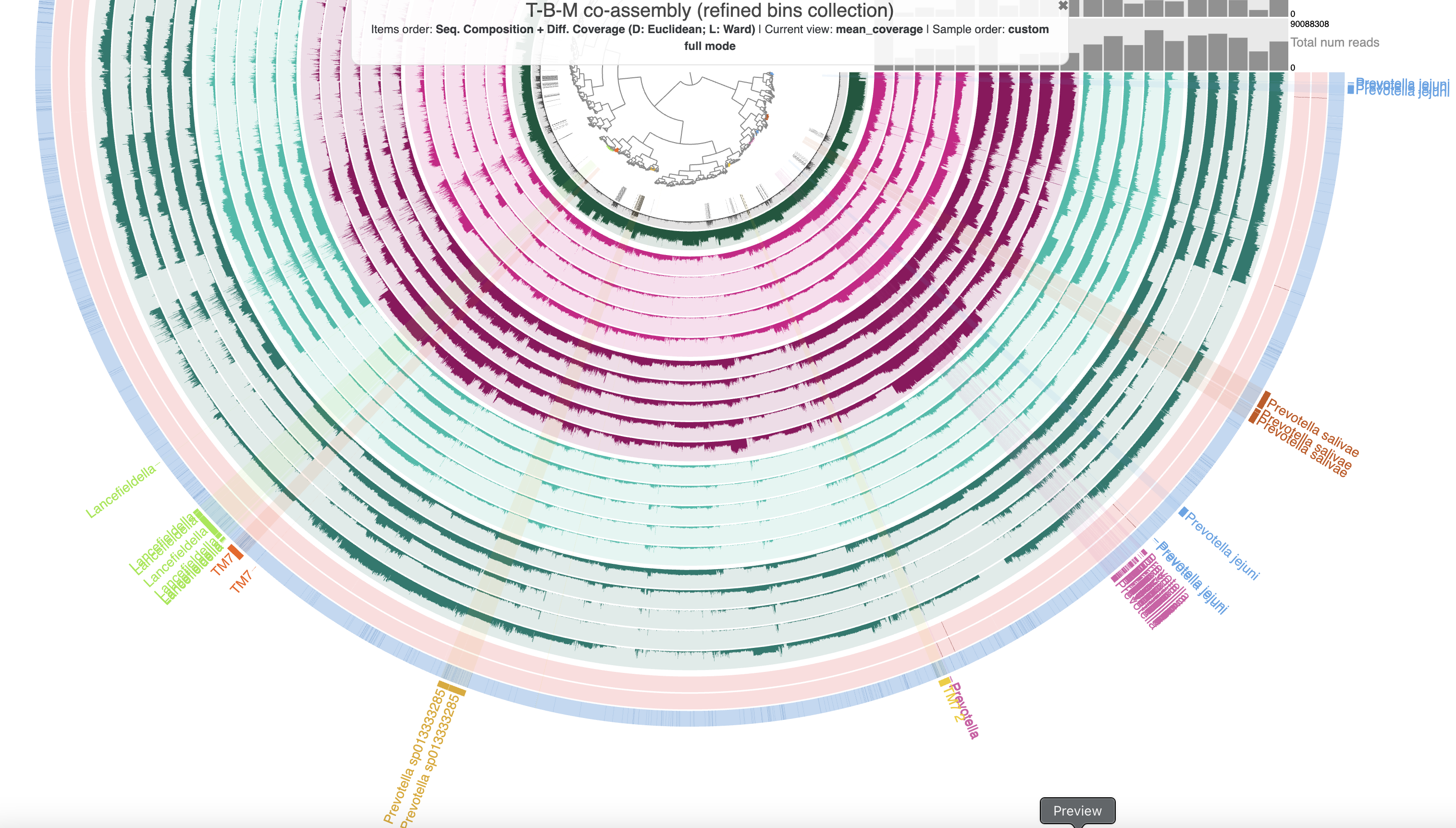
The 7 refined bins in the T-B-M co-assembly.
You can see that most of the refined bins are broken up into several pieces when organized within this larger set of contigs. It is possible that the metabin ‘Bin 3’ was missing pieces of these population genomes, and that by adding the sequences that cluster with these bins, we could increase the bins’ completeness scores. For instance, we could add the missing sequences between the sections of the P. salivae bin – though unfortunately doing this would increase only the size of the bin and not its completeness. There are also some sequences that cluster farther away from the rest of their bin – these could represent potential contaminating sequences that we can now parse out using the additional evidence in this larger figure. For instance, we could remove the split of the TM7 bin that is farther away from the rest – though unfortunately this would not decrease the redundancy of that bin. In both of these examples, since we don’t have changes in the completeness and redundancy estimates to help us track the correctness of our choices, having additional evidence such as gene-level taxonomy or target genome lengths from corresponding reference genomes would be very helpful to justify the additions or removals.
As you can see, visualizing binning results in different contexts and different organizations can be, paradoxically, both confusing and helpful. We could spend ages trying to improve our binning results, and often only see a marginal improvement. Bin refinement is truly an art rather than an exact science. For the sake of this tutorial, we are done here.
Population genetics
Now that we have some manually-refined bins, we can answer our second question: Do the individuals in a couple share similar populations in their oral microbiomes? Now it becomes relevant for you to know that the four individuals represented in our datapack were not chosen randomly – they actually represent two couples. T-B-M is the partner of T-B-F (their sample layers were dark and light green in our interactive interface figures above), and T-A-F is the partner of T-A-M (their samples were the light and dark pink layers). So the question that we want to answer is: are the microbes from T-B-M more similar to the microbes from T-B-F than to either of the communities from T-A-F or T-A-M? We will answer this question using population genetics, whereby we will compare the single-nucleotide variant patterns of a microbial population across different samples to see if the variation is similar between the couples’ samples.
In theory, we could run our comparison using all of the sequence variants in the entire co-assembly, ignoring the boundaries of population genomes and utilizing all the data we have available. But in our case today, we are interested in visualizing the output with the anvi’o interactive interface, and unfortunately that places a limit on the number of variants we can handle (to around 10,000 variant positions). So to reduce the number of variants to a tractable amount, we’ll be focusing on comparing one microbial population across the different samples.
Choosing a population (and samples) to focus on
Which microbial population should we compare? In order to robustly call sequence variants, anvi-profile requires a nucleotide position to have a minimum coverage of 10x (by default). If coverage is less than that minimum threshold at a given position, it won’t identify any single-nucleotide variants (SNVs) at that position. This means that we need a population with enough mean coverage across our samples to be sure that we will have enough variant information for our comparison.
Let’s take a look at the coverage of our refined bins across our samples. If you haven’t already, you can import our refined collection into the contigs database of the datapack:
anvi-import-collection -p PROFILE.db -C refined_Bin_3 refined_Bin_3.txt -c T_B_M-contigs.db
These are the 7 bins we refined from the metabin ‘Bin 3’ in the previous chapter. To get a table of coverage for our bins across samples, we will use the program anvi-summarize:
anvi-summarize -p PROFILE.db -c T_B_M-contigs.db -C refined_Bin_3
Once this command finishes, you should see a new directory of output containing a bunch of summary tables describing our collection of refined bins. Within that directory is a subfolder called bins_across_samples:
ls SUMMARY/bins_across_samples/
In the subfolder’s content list, you should see files with coverage in the name. The mean coverage table (mean_coverage.txt) describes the average coverage across all sequences in a bin within each sample, and the Q2Q3 version (mean_coverage_Q2Q3.txt) does the same thing while ignoring positions with outlier coverage. std_coverage.txt is a table of the standard deviation of the coverage within a bin. We’ll take a look at the mean_coverage_Q2Q3.txt file to get a sense of which microbial populations are consistently well-covered across most samples.
Currently that table has bins in the rows and samples in the columns, which makes it quite wide and unwieldy to look at in the terminal. Let’s quickly transpose that matrix and print it out.
anvi-script-transpose-matrix SUMMARY/bins_across_samples/mean_coverage_Q2Q3.txt -o Q2Q3_transposed.txt
cat Q2Q3_transposed.txt
You should see a table like the following:
| bins | Lancefieldella | Prevotella | Prevotella_jejuni | Prevotella_salivae | Prevotella_sp013333285 | TM7 | TM7_2 |
|---|---|---|---|---|---|---|---|
| T_A_F_01 | 8.624398598160925 | 57.32577760673921 | 74.06072578745524 | 19.911118604245285 | 8.064310610093008 | 9.488094623423084 | 15.545108593218611 |
| T_A_F_02 | 0.015263677285119348 | 1.5420123149848513 | 2.1574547997229856 | 0.2949089576359896 | 0.06715638131320503 | 0.49366065486367816 | 0.9984769300394033 |
| T_A_F_03 | 0.02246682035310184 | 8.101861089789537 | 9.317567758362014 | 1.4602965519362598 | 1.2397849218121701 | 1.778857991981489 | 1.6988925865059272 |
| T_A_F_04 | 0.14188530717151587 | 6.781893936720006 | 7.738333881487812 | 1.0989314577649887 | 0.5857676665668653 | 0.8848732806389906 | 0.9622060591749629 |
| T_A_F_05 | 1.407124426293932 | 28.50991484456179 | 36.46311976385477 | 8.783470983966787 | 3.243910057627215 | 3.3837129889662134 | 2.954984343688233 |
| T_A_M_01 | 29.377456764192477 | 91.63334614727292 | 124.39574466622528 | 41.245129450213 | 11.000324392691299 | 6.18456093548647 | 116.6954863262177 |
| T_A_M_02 | 3.3290187892432197 | 13.110854602630106 | 19.490913999359375 | 4.401445633341987 | 2.085665620813123 | 2.6945818599762634 | 29.841299352291415 |
| T_A_M_03 | 8.56451090767441 | 29.582234936676308 | 42.90967946927104 | 8.379770071964392 | 6.572803564589419 | 4.887071651673707 | 22.33547887845104 |
| T_A_M_04 | 13.3920646601564 | 11.314106440352706 | 23.720177173701227 | 5.0667417594724 | 5.029712971194443 | 2.367945503245309 | 14.930418827409262 |
| T_A_M_05 | 36.290522252746406 | 45.85105409097597 | 53.042064548813826 | 11.248817111954518 | 0.7518639393794053 | 1.7838180122731992 | 4.5802425454302576 |
| T_B_F_01 | 1.7702483684474821 | 1.6027102331849936 | 9.21934644468334 | 1.830647392609952 | 1.3912103628764767 | 1.7416655554709084 | 0.7785042023463407 |
| T_B_F_02 | 1.8205190905809783 | 1.8975659007331909 | 8.869138882987396 | 2.765277634934171 | 1.8410649857385608 | 2.025587164945343 | 1.752652101467555 |
| T_B_F_03 | 0.3962001344383488 | 0.4177397234911995 | 3.8385232774015003 | 0.3662106272303187 | 0.01973096035178188 | 0.2544967083110461 | 0.1993795379423582 |
| T_B_F_04 | 0.6128835782290079 | 0.2518106995967418 | 3.635915600131333 | 0.8019436425672709 | 0.3945328898411596 | 0.9475362090596007 | 0.6832072783089991 |
| T_B_F_05 | 0.19806195248522243 | 0.10907359058908365 | 2.5190935451216 | 0.778226949347181 | 0.035484870038638414 | 0.767851196053339 | 1.0391776169591254 |
| T_B_M_01 | 9.33432544972028 | 4.320107863480356 | 52.34011740514722 | 17.41956809869896 | 6.75780363575873 | 4.960450527533732 | 1.2024745303609714 |
| T_B_M_02 | 4.721418127572123 | 3.6743184761363663 | 50.643042289564306 | 11.992251829114474 | 16.520389700598955 | 9.704686439283101 | 1.7856559495994127 |
| T_B_M_03 | 0.350018524020889 | 0.12942546306354305 | 22.40594596487217 | 0.30016375964763664 | 3.4049773355202486 | 0.009784719222008345 | 0.0 |
| T_B_M_04 | 0.0047172938118133926 | 0.009479416890023894 | 3.8503129305499337 | 0.13539559715154753 | 0.36370656740904705 | 0.004292267768635698 | 0.0 |
| T_B_M_05 | 3.1652843135784403 | 0.16549884178629393 | 27.935287690671082 | 10.579499916252594 | 8.383464218270616 | 1.2780812203044571 | 4.849088857256864 |
Remembering that we want to have a lot of nucleotide positions with at least 10x coverage in order to have decent SNV profiles, what we are looking for is a microbial population that has fairly high overall coverage in as many samples as possible. From this table, it seems clear that none of the microbial populations we binned are going to fit perfectly, since the overall coverages are rather low. But the microbial population with the overall highest coverage is Prevotella jejuni, so that bin will be the target of our population genetics analysis.
Show/Hide Want to look at this table using Python? Click here.
Here is how to load this table in Python and compute the overall mean and median coverage of each bin across all samples.
import pandas as pd
df = pd.read_csv("Q2Q3_transposed.txt", sep="\t", index_col=0)
df.mean()
df.median()
In the results you should see that Prevotella jejuni has the highest mean (and median) coverage across all samples.
You can run these lines of code from the terminal if you start with the command python to open the Python interpreter. When you are done, run exit() to leave the Python interpreter.
You might remember from our binning results that the Prevotella jejuni bin was rather small and incomplete (it didn’t even have any SCGs annotated in it). So in reality, we’ll only be using a subset of the P. jejuni population genome. It is not ideal, but for our particular question it’s more important that we have high enough coverage for proper SNV calling than to have a complete genome.
To that end, we should probably not work with any sample in which the Prevotella jejuni bin has low coverage. We can parse the coverage table to keep only samples in which P. jejuni has a non-outlier mean coverage of at least, let’s say 15x. A mean coverage of 15x doesn’t mean that all nucleotide positions in the bin will have >10x coverage (our minimum threshold for SNV calling), but at least it is likely that a majority of positions will cross that threshold.
To get a list of samples in which this bin has at least 15x mean coverage, we can go back to our coverage table (the table directly in the summary output, SUMMARY/bins_across_samples/mean_coverage_Q2Q3.txt). Below, I export a list automatically using python, but you can feel free to use another way to do it:
import pandas as pd
df = pd.read_csv("SUMMARY/bins_across_samples/mean_coverage_Q2Q3.txt", sep="\t", index_col=0)
df[df > 15].count(axis=1)
df[df > 15].loc['Prevotella_jejuni',].dropna()
samps = df[df > 15].loc['Prevotella_jejuni',].dropna().index.to_list()
with open('samples_of_interest.txt', 'w') as f:
     for s in samps:
             f.write(f"{s}\n")
(A small reminder that you can leave the Python interpreter in the command line by running exit()).
The output we should get is a text file, called samples_of_interest.txt, that contains the 11 samples in which the P. jejuni bin has >15x mean (Q2Q3) coverage. This is what it should look like:
T_A_F_01
T_A_F_05
T_A_M_01
T_A_M_02
T_A_M_03
T_A_M_04
T_A_M_05
T_B_M_01
T_B_M_02
T_B_M_03
T_B_M_05
As you can see, we only have 3 individuals left in our analysis. T-B-F dropped out because P. jejuni didn’t have enough coverage in any of their samples. However, we still have one couple (T-A-F and T-A-M), so we can still take a stab at seeing if these two individuals harbor similar P. jejuni populations.
Let’s move on to the population genetics comparison.
The population genetics part
Now that we know which bin to compare across which samples, we can ask anvi’o to profile the variation for us. Here is the command:
anvi-gen-variability-profile -c T_B_M-contigs.db \
               -p PROFILE.db \
               -C refined_Bin_3 \
               -b Prevotella_jejuni \
               --samples-of-interest samples_of_interest.txt \
               --min-occurrence 5 \
               --min-coverage-in-each-sample 20 \
               --include-split-names \
               --quince-mode \
               -o Prevotella-SNVs.txt
The first few inputs should hopefully be self-explanatory – we provide the co-assembly, the read recruitment information (which includes SNVs that were called by the anvi-profile program during the mapping workflow), our collection of refined bins, the name of the bin that we want to compare, and the list of samples that we selected in the previous section.
The --min-occurrence 5 argument requires that a given SNV position has to be variable in at least 5 samples (out of the 11 samples that we specified in samples_of_interest.txt) in order to be reported. This threshold ensures that we get rid of spurious variants only present in a small fraction of samples that won’t be very useful in our comparison anyway. The --min-coverage-in-each-sample 20 is yet another filter, requiring a variant position to have at least 20x coverage in each sample to be reported. The higher coverage requirement means that when a given position is variable in some samples but not in other samples, we can be sure we aren’t accidentally missing variation in the latter samples just due to low coverage. It also means that when a position is variable, we can be sure it is a true variant and not a random sequencing or alignment error (although the 10x min coverage threshold in anvi-profile should already take care of this to some extent). Both of these filters reduce the number of potential variable positions we will look at, and their goal is to reduce noise.
The other flags control the output of the program. --include-split-names asks for split names to be included in the output variability table, so that we could inspect splits with interesting SNV positions if we wanted to. --quince-mode ensures that each position that is variable in at least 1 sample (by default, or in our case, at least 5 samples due to our use of --min-occurrence 5) will have a corresponding entry from every single sample in the output variability table, even if the position is not variable in some of those samples. As the output file will report variable nucleotide positions on a per-sample basis, you can imagine that ‘Quince mode’ basically completes the matrix of variability across samples – in our case, every position in the co-assembly will have 11 corresponding entries in the output file (one entry for the position’s variation in each of our 11 samples of interest). Finally, -o specifies the name of our output file.
If you run the anvi-gen-variability-profile command, you will see how the filters are working from the output on the terminal. We’ve copied some of the relevant output lines here:
Variability data ..............................................: 9,514,685 entries in 12,499 splits across 11 samples
Entries after split name(s) of interest filter ................: 258,587 (9,256,098 were removed) [320 genes remaining]
Entries after minimum occurrence of positions filter ..........: 224,760 (33,827 were removed) [315 genes remaining]
Entries after quince mode filter ..............................: 281,259 (56,499 were added) [315 genes remaining]
Entries after minimum coverage across all samples filter ......: 109,527 (171,732 were removed) [222 genes remaining]
Num entries reported ..........................................: 109,527
Num NT positions reported .....................................: 9,957
In other words, while there were ~9.5 million SNV positions in the entire T-B-M co-assembly, there were only 258,587 in our Prevotella jejuni bin. When we kept only nucleotide positions that were variable (ie, SNVs at that position) in at least 5 samples, most of them (224,760) remained, which means there were a lot of SNVs that were consistently found across many samples. Filling out the matrix to include an entry for each position in each sample of interest (quince mode) obviously adds a bunch of entries, but many SNV positions drop out due to having <20x coverage in at least one sample.
So we ultimately end up with ~109k entries corresponding to about 10,000 variable nucleotide positions. That’s quite a lot of variation for such a little bin. This population must be quite variable across the different samples (which could include variation over time in one individual and/or variation between the P. jejuni populations living in different hosts).
Let’s take a look at the output. Here are the first 15 rows of the Prevotella-SNVs.txt output file:
| entry_id | unique_pos_identifier | pos | pos_in_contig | split_name | sample_id | corresponding_gene_call | in_noncoding_gene_call | in_coding_gene_call | base_pos_in_codon | codon_order_in_gene | codon_number | gene_length | coverage | cov_outlier_in_split | cov_outlier_in_contig | A | C | G | N | T | reference | consensus | competing_nts | departure_from_reference | departure_from_consensus | n2n1ratio | entropy | kullback_leibler_divergence_raw | kullback_leibler_divergence_normalized |
|---|---|---|---|---|---|---|---|---|---|---|---|---|---|---|---|---|---|---|---|---|---|---|---|---|---|---|---|---|---|
| 0 | 5 | 210 | 210 | c_000000009040_split_00001 | T_A_F_01 | -1 | 0 | 0 | 0 | -1 | 0 | -1 | 74 | 0 | 0 | 0 | 41 | 0 | 0 | 33 | T | C | CT | 0.5540540540540541 | 0.44594594594594594 | 0.8048780487804879 | 0.6872920626194337 | 0.039404109361533976 | 0.035203791606167406 |
| 1 | 5 | 210 | 210 | c_000000009040_split_00001 | T_A_F_05 | -1 | 0 | 0 | 0 | -1 | 0 | -1 | 49 | 1 | 1 | 0 | 20 | 0 | 0 | 29 | T | T | CT | 0.40816326530612246 | 0.40816326530612246 | 0.6896551724137931 | 0.6761830625863905 | 0.16322600016375025 | 0.15567570734592176 |
| 2 | 5 | 210 | 210 | c_000000009040_split_00001 | T_A_M_01 | -1 | 0 | 0 | 0 | -1 | 0 | -1 | 159 | 1 | 1 | 0 | 63 | 1 | 0 | 95 | T | T | CT | 0.4025157232704403 | 0.4025157232704403 | 0.6631578947368421 | 0.7064149414358419 | 0.1770423426114686 | 0.17419681090826308 |
| 3 | 5 | 210 | 210 | c_000000009040_split_00001 | T_A_M_02 | -1 | 0 | 0 | 0 | -1 | 0 | -1 | 37 | 1 | 1 | 0 | 18 | 0 | 0 | 19 | T | T | CT | 0.4864864864864865 | 0.4864864864864865 | 0.9473684210526315 | 0.6927819059876479 | 0.08611588837223735 | 0.08036406987905767 |
| 4 | 5 | 210 | 210 | c_000000009040_split_00001 | T_A_M_03 | -1 | 0 | 0 | 0 | -1 | 0 | -1 | 65 | 0 | 0 | 0 | 38 | 0 | 0 | 27 | T | C | CT | 0.5846153846153845 | 0.4153846153846154 | 0.7105263157894737 | 0.6787585090999517 | 0.024326467528090145 | 0.02082790549105755 |
| 5 | 5 | 210 | 210 | c_000000009040_split_00001 | T_A_M_04 | -1 | 0 | 0 | 0 | -1 | 0 | -1 | 29 | 0 | 0 | 0 | 23 | 0 | 0 | 6 | T | C | CT | 0.7931034482758621 | 0.20689655172413793 | 0.2608695652173913 | 0.5098156995816887 | 0.03219473253455685 | 0.03348351738952218 |
| 6 | 5 | 210 | 210 | c_000000009040_split_00001 | T_A_M_05 | -1 | 0 | 0 | 0 | -1 | 0 | -1 | 53 | 0 | 0 | 0 | 16 | 0 | 0 | 37 | T | T | CT | 0.30188679245283023 | 0.3018867924528302 | 0.43243243243243246 | 0.6124545112186727 | 0.30906205522550045 | 0.29907141962222006 |
| 7 | 5 | 210 | 210 | c_000000009040_split_00001 | T_B_M_01 | -1 | 0 | 0 | 0 | -1 | 0 | -1 | 142 | 1 | 1 | 1 | 136 | 0 | 0 | 5 | T | C | CT | 0.9647887323943662 | 0.04225352112676056 | 0.03676470588235294 | 0.19407878983877083 | 0.25972638102068185 | 0.26957433395305563 |
| 8 | 5 | 210 | 210 | c_000000009040_split_00001 | T_B_M_02 | -1 | 0 | 0 | 0 | -1 | 0 | -1 | 141 | 1 | 1 | 0 | 138 | 0 | 0 | 3 | T | C | CT | 0.9787234042553191 | 0.02127659574468085 | 0.021739130434782608 | 0.10296666046541245 | 0.2956367614999755 | 0.30118779093503445 |
| 9 | 5 | 210 | 210 | c_000000009040_split_00001 | T_B_M_03 | -1 | 0 | 0 | 0 | -1 | 0 | -1 | 29 | 0 | 0 | 0 | 29 | 0 | 0 | 0 | T | C | CC | 1.0 | 0.0 | 0.0 | 0.0 | 0.3821654642801116 | 0.3882050513943119 |
| 10 | 5 | 210 | 210 | c_000000009040_split_00001 | T_B_M_05 | -1 | 0 | 0 | 0 | -1 | 0 | -1 | 28 | 1 | 1 | 0 | 28 | 0 | 0 | 0 | T | C | CC | 1.0 | 0.0 | 0.0 | 0.0 | 0.3821654642801116 | 0.3882050513943119 |
| 11 | 6 | 217 | 217 | c_000000009040_split_00001 | T_A_F_01 | -1 | 0 | 0 | 0 | -1 | 0 | -1 | 74 | 0 | 0 | 1 | 36 | 2 | 0 | 35 | C | C | CT | 0.5135135135135135 | 0.5135135135135135 | 0.9722222222222222 | 0.8604143053978275 | 0.10146204711563164 | 0.09318172894505758 |
| 12 | 6 | 217 | 217 | c_000000009040_split_00001 | T_A_F_05 | -1 | 0 | 0 | 0 | -1 | 0 | -1 | 51 | 1 | 1 | 0 | 36 | 0 | 0 | 15 | C | C | CT | 0.2941176470588235 | 0.29411764705882354 | 0.4166666666666667 | 0.605797499372304 | 0.30224048427639116 | 0.2588360551347535 |
| 13 | 6 | 217 | 217 | c_000000009040_split_00001 | T_A_M_01 | -1 | 0 | 0 | 0 | -1 | 0 | -1 | 167 | 1 | 1 | 1 | 91 | 1 | 0 | 74 | C | C | CT | 0.45508982035928147 | 0.4550898203592814 | 0.8131868131868132 | 0.7527900280446478 | 0.10431591683037689 | 0.08234652861536867 |
The columns in this output file have been explained elsewhere, so we won’t repeat ourselves here. You can at least notice that we have 11 entries for the same nucleotide position (position 210 in the table), which is due to the quince mode filter. This position is a T in the co-assembly contig sequence, but most of the samples have at least a portion of reads mapping to the position that have a C nucleotide instead – in fact, C is the consensus nucleotide in samples like T_A_F_01, T_A_M_03, T_A_M_04, and all of the T_B_M samples. The changing consensus base in some samples suggests that the variation at this particular position changed over time in the individuals T-A-F and T-A-M, but as far as we know (from the samples we were able to include), it mostly stayed stable with a majority C base in the individual T-B-M.
Of course, manually examining all variable positions is not a tractable strategy to compare our samples. Ideally we would like to visualize the results to answer our target question.
Visualizing the variable positions
The SNV interactive interface
First, let’s do it using the anvi’o interactive interface. We can do this by converting our variability table into a view-data file, which just means a tab-delimited text file that the interactive interface can read from in --manual mode, and in this particular case will make the variable nucleotide positions into ‘items’ and decorating information about its variation in different samples into the ‘layers’.
Luckily, there is already a program that will consolidate and reformat our variability table for us, then create a profile database with a nice organization of the variable positions:
anvi-script-snvs-to-interactive Prevotella-SNVs.txt -o Prevotella-snvs
Note that this script by default makes the departure_from_consensus column the value shown in the interactive interface for each position. This helps you distinguish between positions that are extremely uniform within a given sample and those that are extremely variable. If you want to visualize the departure_from_reference values instead (to identify at which positions the short reads do not agree with the reference assembly), you can use the parameter --display-dep-from-reference.
We can then visualize the variable positions by running the following command:
anvi-interactive --manual -p Prevotella-snvs/profile.db \
                 --tree Prevotella-snvs/tree.txt \
                 --view-data Prevotella-snvs/view.txt \
                 --title "P. jejuni variable positions"
There is a technical limit to the number of variable positions that can be shown in the anvi’o interactive interface in this way (similar to how there is a limit for the number of splits when visualizing an assembly). We are below the limit in our case, but if you end up passing that limit when using your own data, you’ll either need to filter out more positions to get below the limit, find an alternative way to visualize the data, or analyze the variability table without visualizing it.
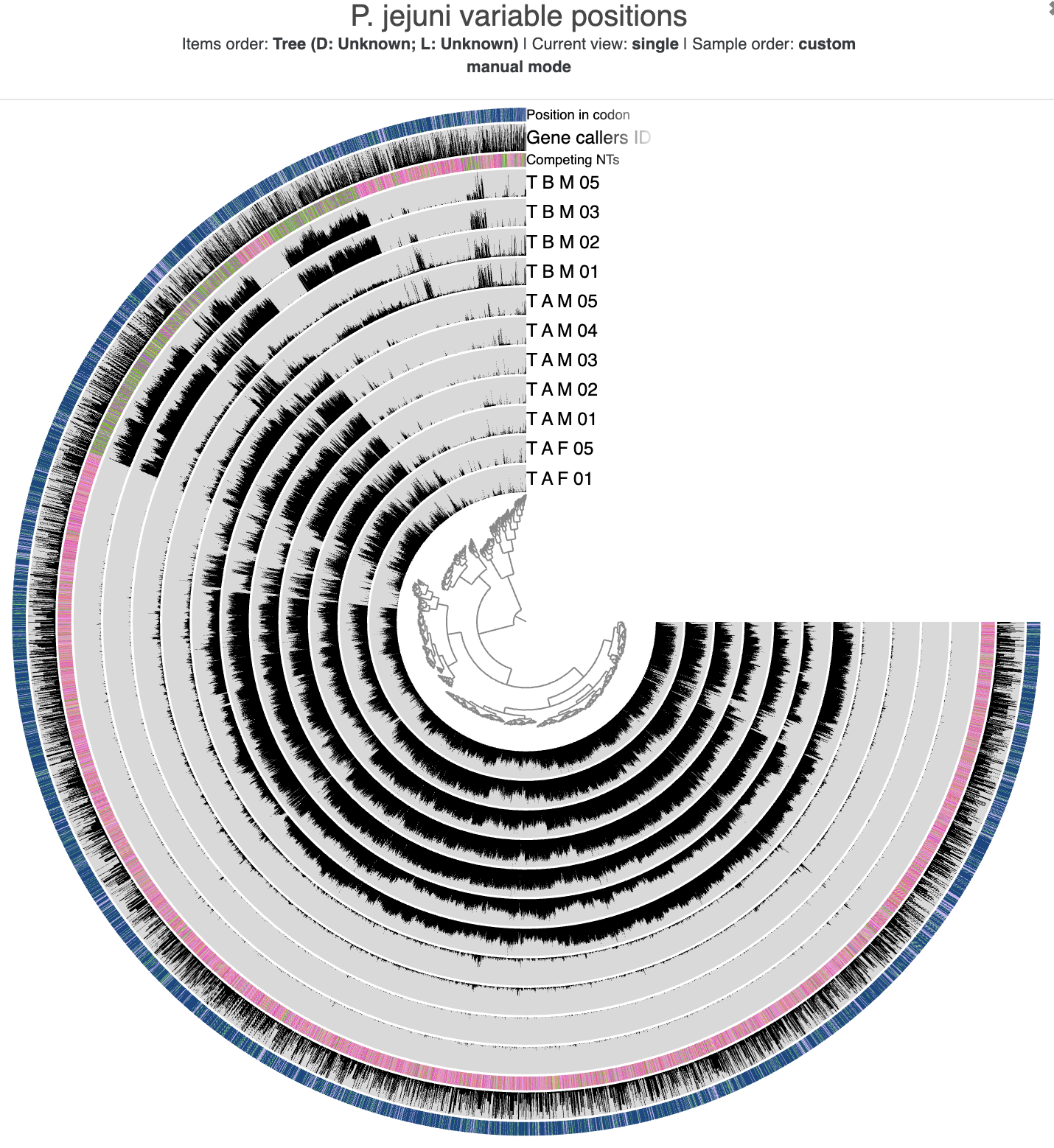
The initial SNV interactive interface.
The main layers of this interface show the departure_from_consensus value for each position in each sample that we analyzed. We also get layers to show the competing nucleotides, the corresponding gene caller ID (if the position is within a gene call), and its relative position within a codon (again, if it is within a protein-coding gene) for each variable position.
But currently the interface isn’t really pretty. Let’s make it match the colors from our co-assembly so that we can more easily distinguish between samples from different individuals (and different couples).
To do this, we’ll export the visualization settings from the co-assembly’s profile database, and import those settings into this profile database:
anvi-export-state -p PROFILE.db -s default -o default.json
anvi-import-state -p Prevotella-snvs/profile.db -n default -s default.json
Then we can simply re-run the interactive command:
anvi-interactive --manual -p Prevotella-snvs/profile.db \
                 --tree Prevotella-snvs/tree.txt \
                 --view-data Prevotella-snvs/view.txt \
                 --title "P. jejuni variable positions"
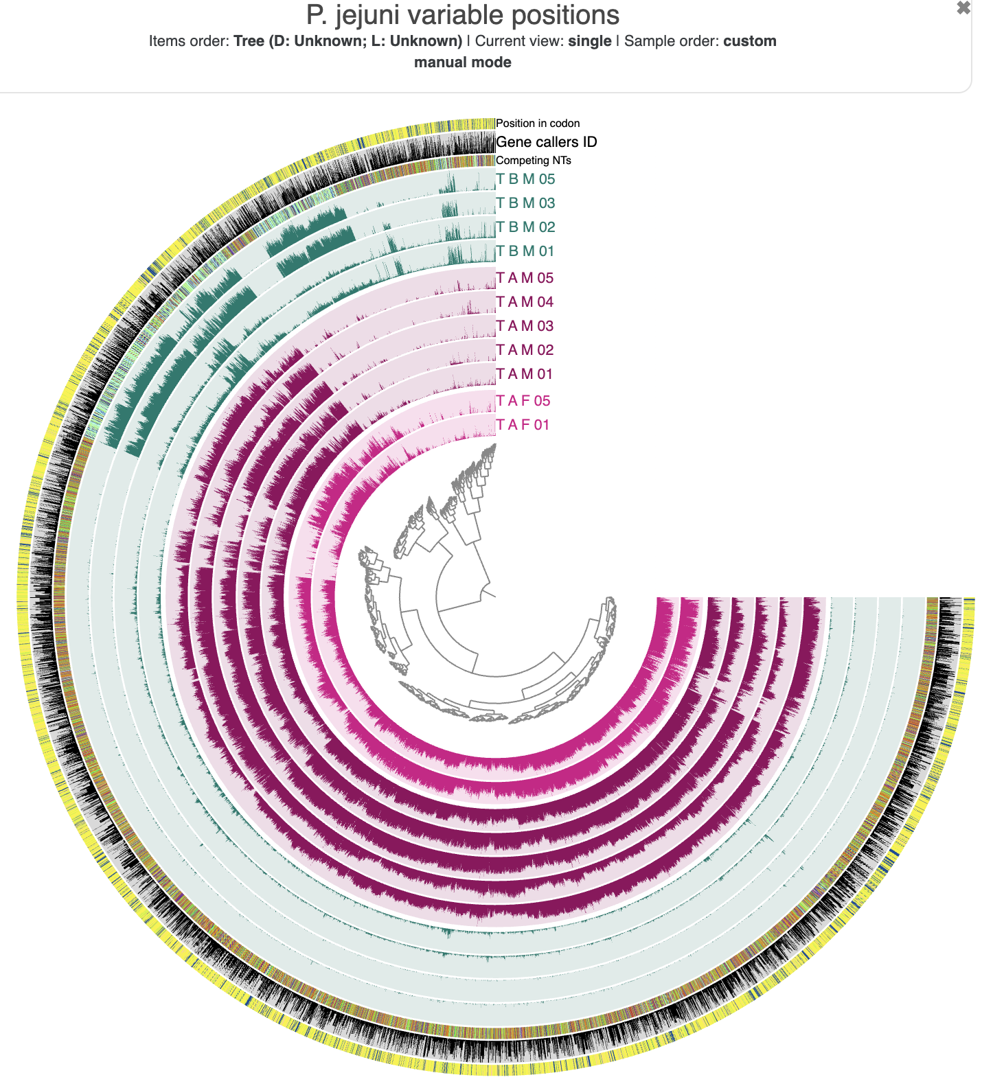
A much prettier version of the SNV interactive interface.
Much better. Now it is extra clear that the different individuals have distinct versions of the P. jejuni population. In particular, there is not as much variation in the dark green T-B-M samples, which makes sense because this is the population that we have binned from the T-B-M co-assembly. The positions that do vary in this individual generally seem to agree with each other (low departure from consensus) at time points 1 and 2, meaning that there isn’t much subpopulation variation in this individual at that time. But this seems to have shifted after time point 3, at which point extensive subpopulation variation of P. jejuni appeared.
We can also see that there is high departure from consensus in the samples from the two other (partnered) individuals, and more importantly, that these variable positions clearly match across those two individuals with a similar amount of departure from consensus. So we know that they are different from the consensus at these positions, but we don’t yet know if their specific nucleotides match between T-A-F samples and T-A-M samples. So we don’t quite have have an answer to our question just yet.
Fixation index to compare samples
To confirm whether the P. jejuni populations are similar between T-A-F and T-A-M, we can compute a matrix of fixation index instead, and automatically cluster this matrix to group similar samples together.
Let’s do it. All we need is to pass the variability table to anvi-gen-fixation-index-matrix, cluster the output matrix to get a dendrogram in Newick format, and open the dendrogram in the interface:
anvi-gen-fixation-index-matrix --variability-profile Prevotella-SNVs.txt \
                               --output-file FST_Prevotella.txt
anvi-matrix-to-newick FST_Prevotella.txt -o FST_Prevotella.nwk
anvi-interactive -t FST_Prevotella.nwk \
                 -p FST_Prevotella.db \
                 --manual
After a bit of fussing with the interface settings to convert the sample names into text (instead of the default colors), and binning the samples from individual T-B-M, you could see a tree that looks like the following:
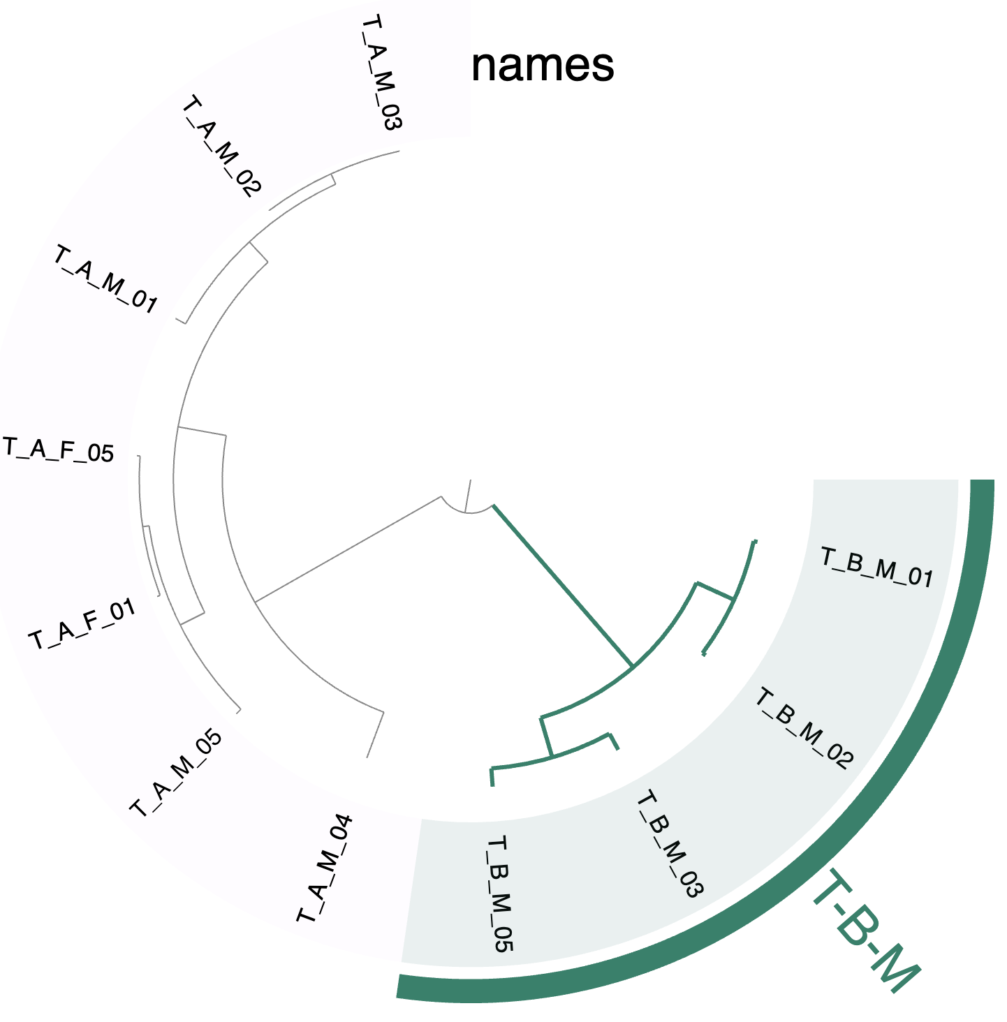
The fixation index tree.
So, now we have our answer :) The samples from couple ‘A’ do truly share similar P. jejuni populations, which are distinct from the P. jejuni living in our individual from couple ‘B’.
A network visualization
Another way of displaying the same data would be to compute a network, where variable positions are small nodes, and each sample is a big node, and the big nodes are connected via edges to small nodes if the corresponding position is variable in the corresponding sample. Visualizing such a network is another strategy to answer the question of ‘which samples come together based on having similar P. jejuni populations’, like we did with the fixation index tree, but this time you’d also be able to see the SNVs that bring the samples together. And – you guessed it – we have a helper program in anvi’o to get you the proper network file.
Here is the command to convert the variability table into a graph file that is compatible with the network visualization software Gephi:
anvi-gen-variability-network -i Prevotella-SNVs.txt \
                             -o Prevotella-SNVs.gexf
If you open that file in the Gephi software, you can choose the ‘Force Atlas 2’ option in the ‘Layout’ panel on the left side, and hit the ‘Run’ button so that it computes an optimal arrangement of the nodes and edges in the network.
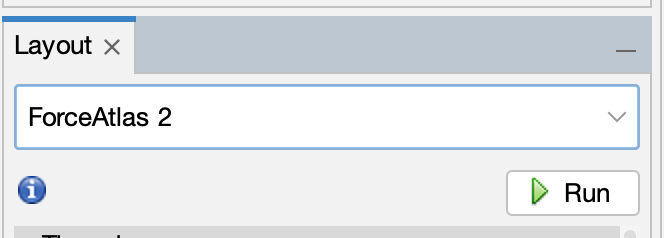
The Force Atlast 2 layout option for visualizing the network.
We also recommend turning on the options ‘LinLog mode’ and ‘Prevent Overlap’ to make the network even easier to read. Once the layout algorithm has run for a bit and hopefully reached some sort of consensus arrangement, you can hit ‘Stop’ in the ‘Layout’ panel, and switch to the ‘Preview’ tab to view the final visualization. You can turn on the ‘Show Labels’ option and turn off the ‘Show Edges’ option in the settings on the left side to make it look less like a crazy spiderweb and more like a somewhat organized collection of named dots.
The network visualization should hopefully look similar to this one:
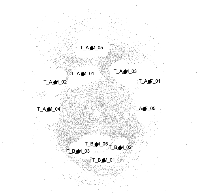
Our Gephi visualization of the P. jejuni SNV network.
As you can see, once again the samples from the ‘A’ couple loosely group together, and are clearly distinct from the samples of our T-B-M individual.
Conclusion
In our small yet realistically-complex tongue microbiome datapack, we’ve been able to achieve our two goals. We refined 7 bins from one CONCOCT metabin, including population genomes of expected oral microbes like TM7 and Prevotella. And, we used one of those refined bins to prove that humans in long-term relationships with each other share similar oral microbiota – the reasons for this are likely obvious to you, but now you can see the proof with your own eyes. ;)
We hope this little tutorial helped to demonstrate the reality of metabin refinement and the utility of population genetics to answer a realistic biological question. If you have any questions or suggestions, let us know in the comments.