Leveling up pangenomics with interactive pangenome graphs

Table of Contents
The purpose of this tutorial is to familiarize you to the upcoming anvi’o pangenome graphs framework, with which you can,
- Identify and analyse regions of hypervariability in your genomes,
- Estimate similarity between the genomes based on graph structures instead of e.g. genome similarity,
- Interactively visualize your pangenome graph and the impact of single genomes on the consensus graph,
- Highlight the distribution of paralogous gene clusters through their synteny-based subclusters,
- Summarize distribution and frequency of common graph motifs into a nice table for downstream analysis, and,
- Create paper-ready visualizations of gene synteny structures not visualizable with other tools.
You can use the anvi’o tutorial for pangenome graphs even if you haven’t done any metagenomic work with anvi’o. All you need is an anvi’o installation, and a FASTA file for each of your genomes.
Introduction
This tutorial will walk you through the following steps:
- Download and order a four genome dataset containing complete and draft genomes using anvi-reorient-contigs,
- Use anvi-run-workflow to generate an anvi’o genomes-storage-db and pan-db,
- Define a subset of genomes for further analysis anvi’o interactive interface enabled by ,
- Survey the genomes using anvi-display-pan and identify a subset for further analysis,
- Generate an anvi’o pangenome graph using anvi-pan-graph
- Explain common graph motifs in the anvi’o interactive interface using anvi-display-pan-graph.
The anvi’o framework for pangenome graphs is still in development. Your input and suggestions are most welcome, and Alex thanks you in advance for your patience if/when occasional bugs appear out of nowhere :)
Setting the stage
The following steps will set the stage for us to jump into the action by ensuring that your computer is ready to generate pangenome graphs, and you have the necessary files in the right place.
Anvi’o dependencies
If your system is properly setup, this anvi-self-test command should run without any errors:
conda activate anvio-dev
anvi-self-test --suite pangenomics
Anvi’o might complain in case you haven’t set up the databases yet and we strongly advise you to do so before running this tutorial.
anvi-setup-scg-taxonomy
anvi-setup-ncbi-cogs
anvi-setup-kegg-data
Changing the branch
Anvi’o pangenome graph is currently only available in a seperate branch of the development version of anvi’o.
cd ~/github/anvio
git checkout pangraph-0.3.0
git pull
cd anvio/data/interactive
npm i
Please note that you will need to remember to switch back to the master branch once you are done here, and you can run the following command to do that when you are ready (don’t do it now though):
cd ~/github/anvio
git checkout master
Obtaining the data
For this workflow we will use four novel and complete genomes from a SAR11 clade that is recently named as Ampluspelagibacter kiloensis by Kelle Freel et al..
A pangenome graph analysis can also be performed with draft genomes, as long as one complete genome is available. But a dataset of complete genomes gives the best results, so we take advantage of that for the sake of this tutorial.
Before we start, let’s first create a specific directory for this tutorial to keep things neatly together.
# create a new directory for this tutorial in your home directory
mkdir ~/PANGENOME-GRAPHS-TUTORIAL/

# go into the newly created directory
cd ~/PANGENOME-GRAPHS-TUTORIAL/
Assuming that we are not in the directory in which you wish to follow this tutorial, we are ready to download all six genomes:
curl -L https://cloud.uol.de/public.php/dav/files/dj83fattaQjq6zB \
     -o original_files.tar.gz
tar -zxvf original_files.tar.gz && rm original_files.tar.gz
The current folder structure should look like this.
~/PANGENOME-GRAPHS-TUTORIAL/
    └── original_files/
        ├── HIMB1526.fa
        ├── HIMB1552.fa
        ├── HIMB1556.fa
        ├── HIMB1636.fa
        ├── HIMB1641.fa
        └── HIMB1702.fa
Processing draft genomes
In the next step we have to order and reorient the contigs of the genomes. Even if we have only complete genomes it is a good idea to run this step, as it defines one direction for all the genomes in the dataset. We use the program anvi-reorient-contigs for this task, based on the longest complete genome present in our folder.
This step is necessary for the pangenome graph creation to make sure the gene synteny matches between the genomes.
mkdir reoriented_files
anvi-reorient-contigs --input-dir original_files/ --output-dir reoriented_files/ --prioritize-genome-size
The fasta files containing draft genomes are now ready to be used on the pangenomics workflow. For every genome excluding the leading genome we see some blast result files in the folder, that were used for reorienting based on the most complete genome.
~/PANGENOME-GRAPHS-TUTORIAL/
    ├── original_files/
        ├── HIMB1526.fa
        ├── HIMB1526-blast.xml
        ├── HIMB1552.fa
        ├── HIMB1552-blast.xml
        ├── HIMB1556.fa
        ├── HIMB1556-blast.xml
        ├── HIMB1636.fa
        ├── HIMB1636-blast.xml
        ├── HIMB1641.fa
        ├── HIMB1641-blast.xml
        └── HIMB1702.fa
    └── reoriented_files/
        ├── HIMB1526.fa
        ├── HIMB1552.fa
        ├── HIMB1556.fa
        ├── HIMB1636.fa
        ├── HIMB1641.fa
        └── HIMB1702.fa
If you are here, you are ready to start the analysis!
Generating a pangenome
From the workflow we will receive multiple databases that we need for further downstream analysis. A single contigs-db for every genome used, containing information like gene calls, annotations, etc. The genomes-storage-db is a special anvi’o database that stores information about genomes, and can be generated from external-genomes, internal-genomes, or both. And lastly the pan-db created from the genomes-storage-db includes all features calculated during the pangenomics analysis. For a more detailed description of these special anvi’o databases please read about it in the anvi’o pangenomics workflow.
For the anvi’o pangenomics workflow we need to first describe the location of our FASTA files through a fasta-file file. This file has to be tab-seperated with two columns, the first containing the name of the fasta and the second containig the path to the file. We use the power of bash to speed things up a little. For more information about anvi’o workflows in general we really recommend reading Scaling up your analysis with workflows.
It has to look similar to this file similar to this one with complete paths to every fasta file we use in the analysis.
name	path
HIMB1526    /home/user/PANGENOME-GRAPHS-TUTORIAL/reoriented_files/HIMB1526.fa
HIMB1552    /home/user/PANGENOME-GRAPHS-TUTORIAL/reoriented_files/HIMB1552.fa
HIMB1556    /home/user/PANGENOME-GRAPHS-TUTORIAL/reoriented_files/HIMB1556.fa
HIMB1636    /home/user/PANGENOME-GRAPHS-TUTORIAL/reoriented_files/HIMB1636.fa
HIMB1641    /home/user/PANGENOME-GRAPHS-TUTORIAL/reoriented_files/HIMB1641.fa
HIMB1702    /home/user/PANGENOME-GRAPHS-TUTORIAL/reoriented_files/HIMB1702.fa
You can create this file using EXCEL or any other text editor, copy it from here and replace user with your user name or use the following quick and hacky bash loop to read the files in the folder and write the full paths into a new file.
echo -e 'name\tpath' > fasta.txt
for filename in *.fna; do
    echo -e $(basename $filename | cut -d. -f1)'\t'$(realpath $filename) >> fasta.txt
done
Now the first prerequisite to start the anvi’o pangenomics workflow is set-up. The next step is to generate and modify the workflow-config. We can create a standard one with this command.
anvi-run-workflow -w pangenomics --get-default-config config.yaml
For the sake of simplicity we will keep most values as they are. The only changes we make are on the bottom of the workflow-config by changing the name of the project and add an output path for the external-genomes, because we need this file later.
config.yaml:
{...}
    "project_name": "Ampluspelagibacter_kiloensis",
    "internal_genomes": "",
    "external_genomes": "external-genomes.txt",
    "sequence_source_for_phylogeny": "",
    "output_dirs": {
        "FASTA_DIR": "01_FASTA",
        "CONTIGS_DIR": "02_CONTIGS",
        "PHYLO_DIR": "01_PHYLOGENOMICS",
        "PAN_DIR": "03_PAN",
        "LOGS_DIR": "00_LOGS"
    },
    "max_threads": "",
    "config_version": "3",
    "workflow_name": "pangenomics"
}
Now we can start the anvi’o pangenomics workflow. This will probably take a while and you can reward yourself with a coffee while you wait ☕
anvi-run-workflow -w pangenomics -c config.yaml
The final command of this section will be to calculate the ANI of our dataset with the program anvi-compute-genome-similarity, which uses various tools such as PyANI to compute average nucleotide identity, followed by sourmash to compute mash distance across our genomes. We use it now to add these results as an additional data layer to our pangenome. More information on ANI and the usage in comparative genomics can be found in the tutorial on pangenomics in the section Computing the average nucleotide identity for genomes. Since our genomes are quite similar it should not take longer than a minute.
anvi-compute-genome-similarity --external-genomes external-genomes.txt \
                               --program pyANI \
                               --output-dir 04_ANI \
                               --num-threads 6 \
                               --pan-db 03_PAN/Ampluspelagibacter_kiloensis-PAN.db
Good job, 5 points for insert your hogwarts house here!
Your folder structure should look similar to this.
~/PANGENOME-GRAPHS-TUTORIAL/
    ├── 00_LOGS/
        └── ...
    ├── 01_FASTA/
        └── ...
    ├── 02_CONTIGS/
        ├── HIMB1526-contig.db
        ├── HIMB1552-contig.db
        ├── HIMB1556-contig.db
        ├── HIMB1636-contig.db
        ├── HIMB1641-contig.db
        ├── HIMB1702-contig.db
        └── ...
    ├── 03_PAN/
        ├── Ampluspelagibacter_kiloensis-GENOMES.db
        ├── Ampluspelagibacter_kiloensis-PAN.db
        └── ...
    ├── 04_ANI/
        └── ...
    ├── original_files/
        └── ...
    ├── reoriented_files/
        └── ...
    ├── config.yaml
    ├── external-genomes.txt
    └── fasta.txt
Generating a pangenome graph
Subsetting the genomes for pangenome graph
We first run the anvi’o interactive interface with anvi-display-pan to visualize our pangenome.
In case you don’t want to wait for a whole pangenome to run, you can just download the folder at this stage from the University of Oldenburg cloud.
mkdir ~/PANGENOME-GRAPHS-TUTORIAL/

curl -L https://cloud.uol.de/public.php/dav/files/CPdpXLNWHwSKTfR \
     -o ~/PANGENOME-GRAPHS-TUTORIAL/AMPLUSPELAGIBACTER-ANVIO-FILES.zip

cd ~/PANGENOME-GRAPHS-TUTORIAL/

unzip AMPLUSPELAGIBACTER-ANVIO-FILES.zip
anvi-display-pan -p 03_PAN/Ampluspelagibacter_kiloensis-PAN.db \
                 -g 03_PAN/Ampluspelagibacter_kiloensis-GENOMES.db
In case this is your first time opening a pangenome, reading the anvi’o pangenomics workflow might be beneficial to you as we won’t go into detail on pangenomes here and having some experience on them will help you in the later part of this tutorial.
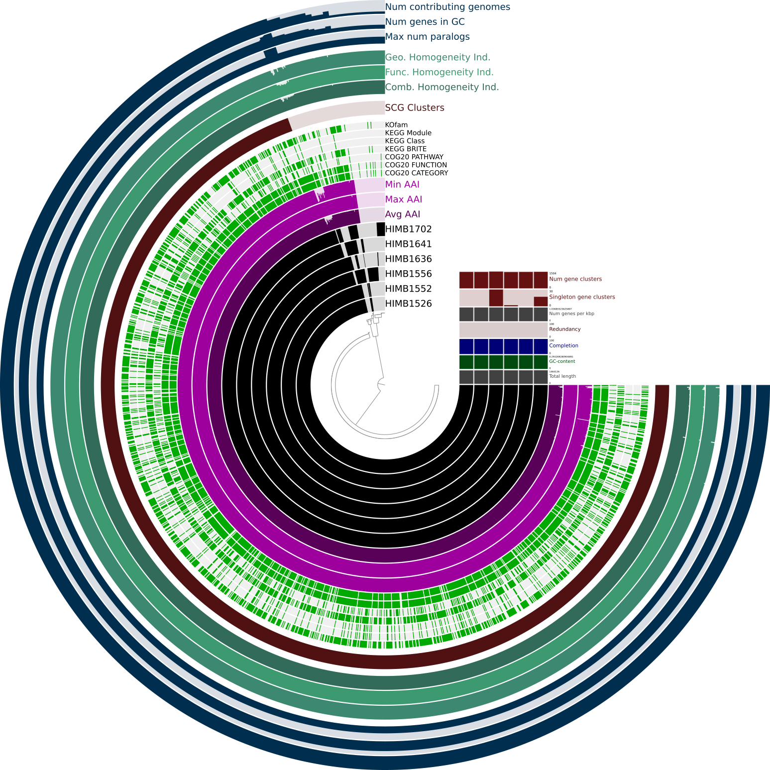
After you click on the draw button you should see a pangenome that looks somewhat similar to this. We strongly recommend to use Google Chrome to offer you the best possible user experience.
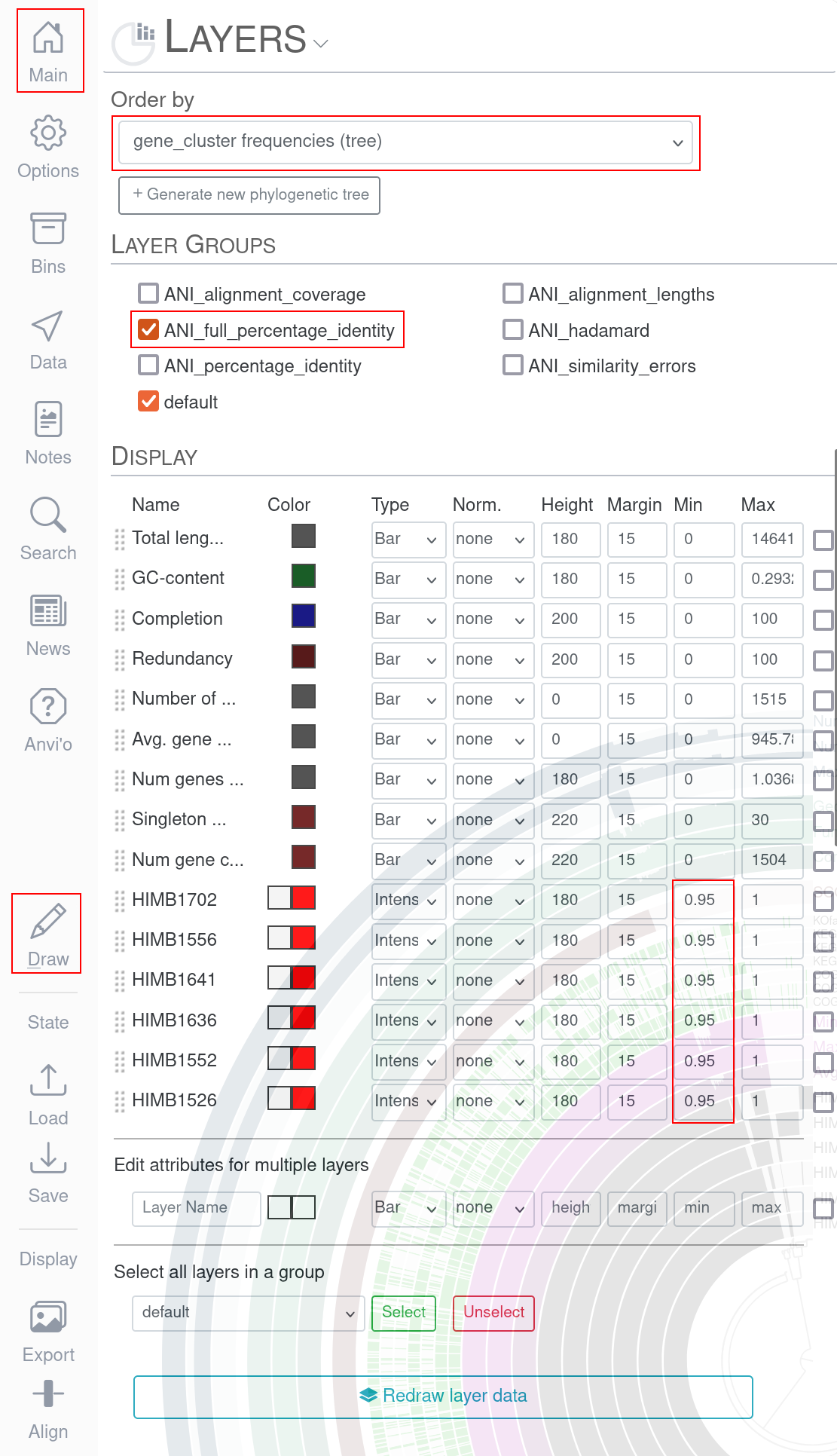
In the Main tab under Layers we first order by gene_cluster_frequencies. In Layer Groups you checkmark the entry ANI_full_percentage_identity and in Display you change the bottom four entries to Bar and the Min value to at least 0.95.
After pressing the draw button again, the resulting pangenome should look like this.
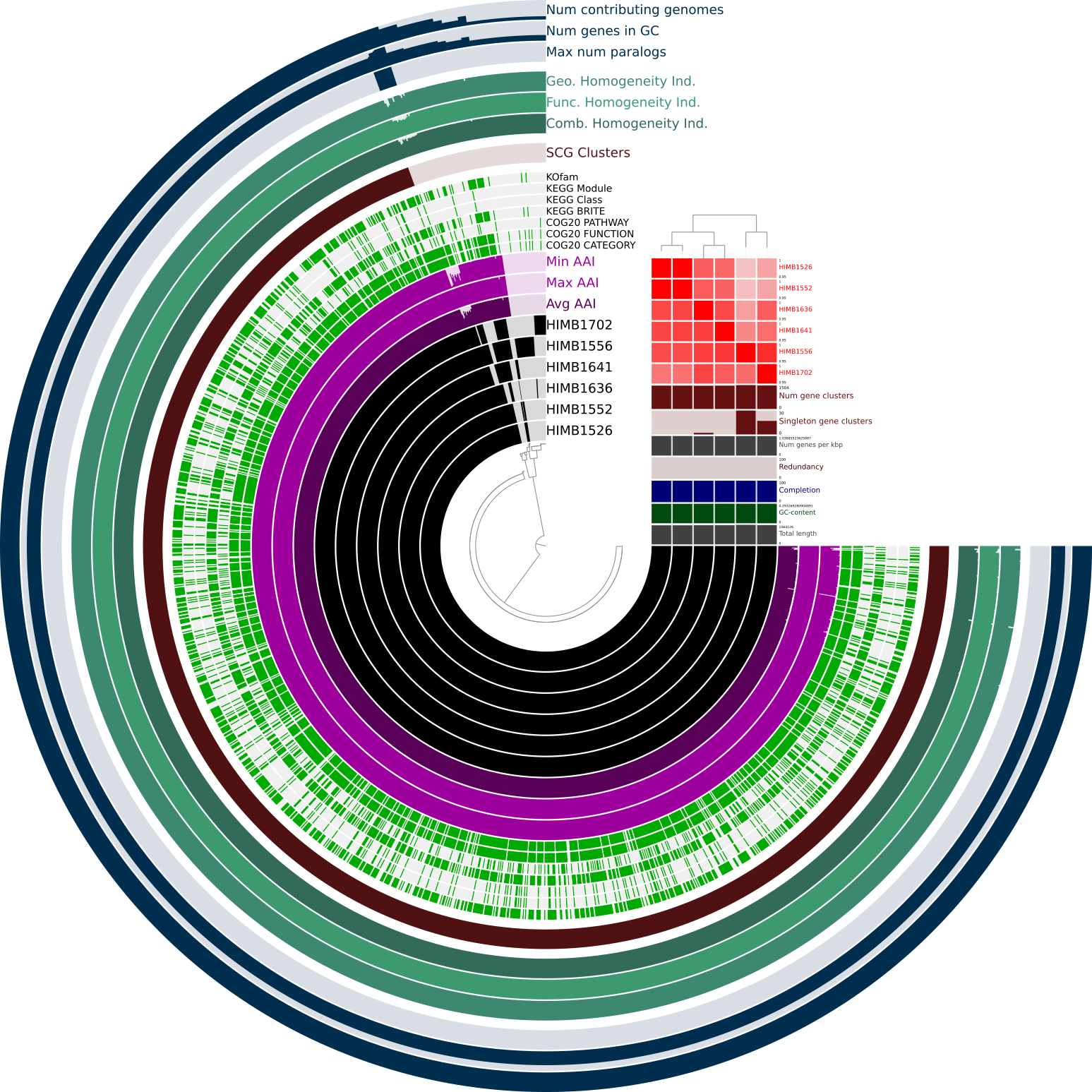
In the newly added red squares we see the ANI between the genomes of the pangenome. Aside from the diagonal which contains a similarity of 100% due to comparing the same genomes with each other, we see a second very high ANI square on the top left. The genome HIMB1526 shares a very high ANI with the genome HIMB1552.
Creating an anvi’o pangenome graph
To follow the anvi’o naming standard we first create a folder named 05_PANGRAPH.
mkdir 05_PANGRAPH
Anvi’o pangenome graphs are then created by the command anvi-run-pangraph. Instead of a genomes-storage-db or pan-db, the result is written in a JSON file in the current version.
anvi-pan-graph --pan-db 03_PAN/Ampluspelagibacter_kiloensis-PAN.db \
               --genomes-storage 03_PAN/Ampluspelagibacter_kiloensis-GENOMES.db \
               --external-genomes external-genomes.txt \
               --project-name 'Ampluspelagibacter_kiloensis' \
               -o 05_PANGRAPH/ \
               --output-pangenome-graph-summary \
               --output-synteny-distance-dendrogram \
               --circularize
Opening the anvi’o interactive interface functions similarly to the one we used before to inspect the pangenome. Instead of anvi-display-pan, we use the program anvi-display-pan-graph. Experienced anvi’o users should feel right at home here and find many functions they already know.
anvi-display-pan-graph -i 05_PANGRAPH/Ampluspelagibacter_kiloensis-JSON.json \
                       -p 03_PAN/Ampluspelagibacter_kiloensis-PAN.db \
                       -g 03_PAN/Ampluspelagibacter_kiloensis-GENOMES.db
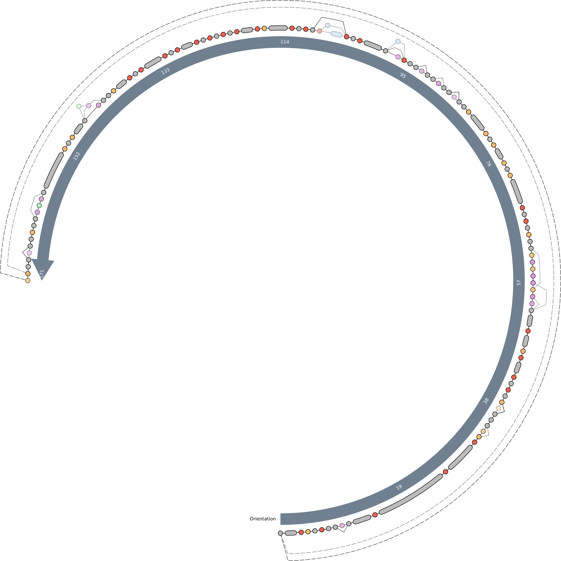
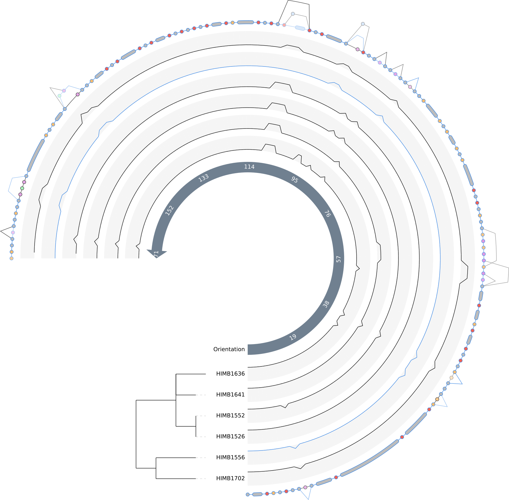
The initial pangenome graph visible in the anvi’o interactive interface should look like this. The grey nodes are single gene clusters (you can click on them to get detailed information on the gene). The purple colored nodes are gene cluster groups, which are created if a set of single gene clusters is only connected in a single line and present in the same subset of genomes. Gene cluster groups basically help to focus on the interesting parts of a pangenome graph. You can also get a detailed view on them by clicking. In the middle you see a arrow showing the graph’s flow direction. There are three different types of edges currently implemented in the pangenome graph tool:
- straight lines [───────]: Those are connections between two gene clusters of gene cluster groups following the pangenome graphs flow direction
- dashed lines [─ ─ ─ ─]: These are like straight lines but reverse the pangenome graph flow direction
- semi-dashed-lines [──── ──]: These are special and sometimes hard to see, because these are a mix between both of the prior edge types. Imagine a situation where a set of genes is reversed all together in a subset of the genomes. Therefore A - B - C is as correct as C - B - A. We implemented this solution to not overload the graph with extra lines. Unfortunately there is no example in the graph below as they occur very rarely and only in VERY complex pangenome graphs.
The consensus graph present to you now already tells us many stories, e.g. insertions and deletions of single genes or potentially full operons. To highlight the genome these events take place in, we will change some settings.
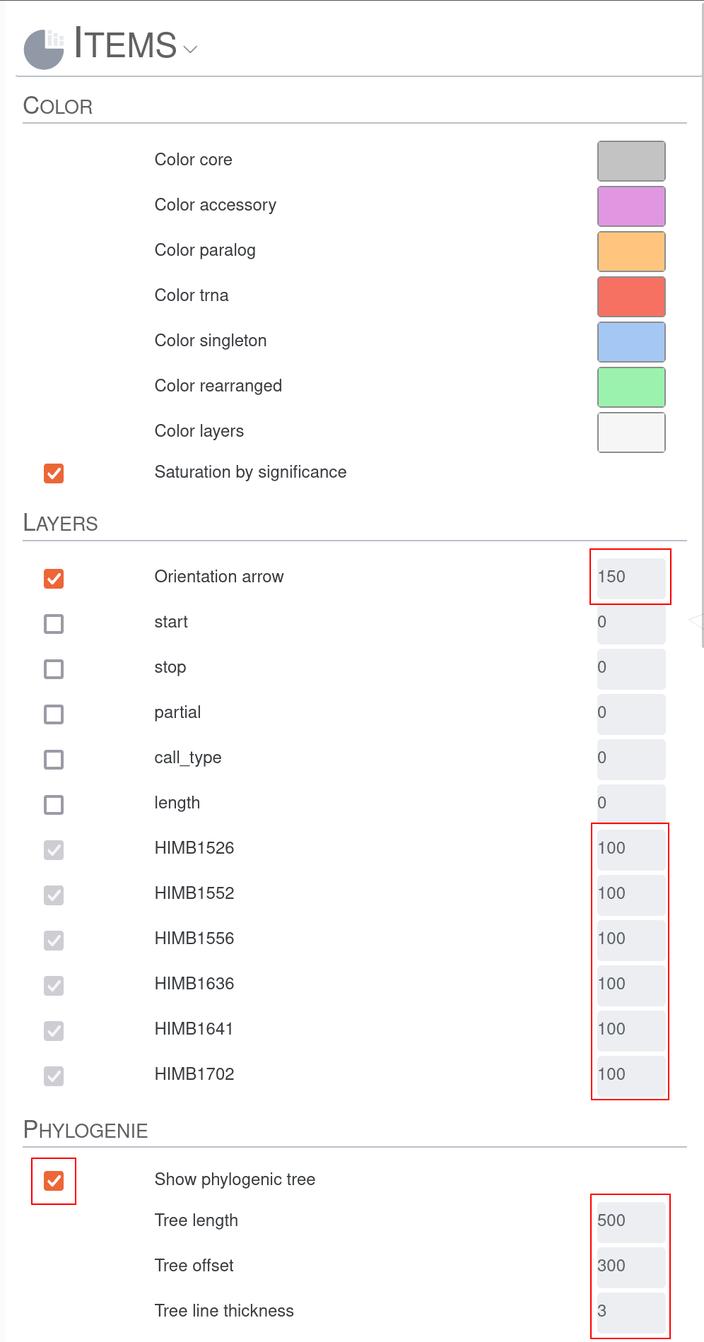
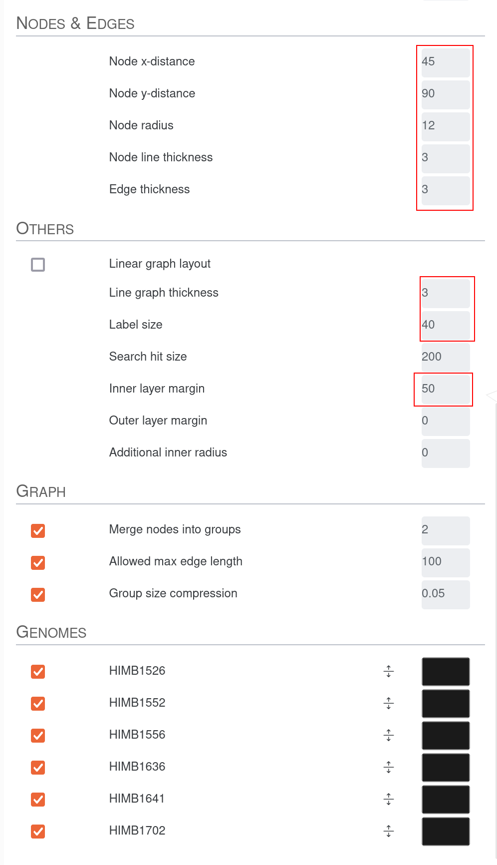
First we increase the size of the Orientation arrow and activate the layers for the two genomes. We also increase them in size. To see the tree based on graph difference we checkmark Show phylogenic tree and increase the size of Tree length and Tree offset. The distance between the nodes on the consensus graph can also be slightly increased. To be able to see the lines in the genome tracks and in the consensus graph we also slightly increase Node line thickness and Edge thickness as well as Line graph thickness. Since we increased the Tree offset, we have more space for labels; therefore, we can increase the Label size. To estimate the size of groups of genes we set the Group size compression to a small value above 0. F
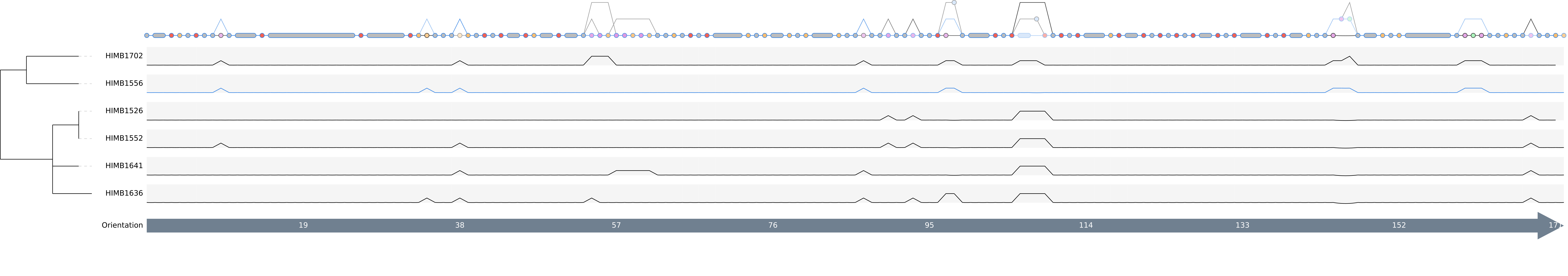
After clicking the Draw button again we should be able to see the so-called “genome tracks” in the middle of the pangenome graph to help us understand the origin of specific motifs.
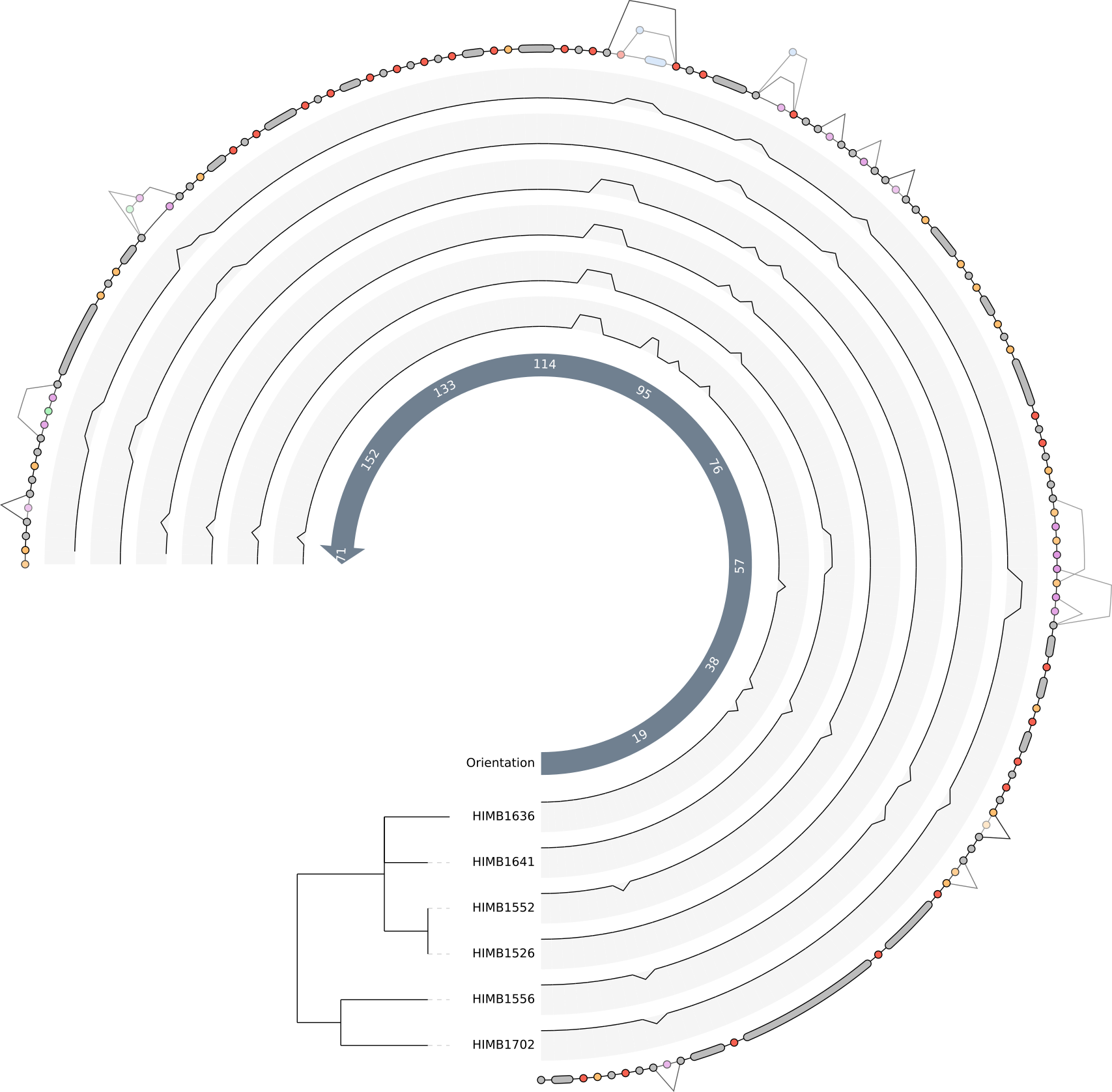
We can now decide if the graph is simple enough to understand, and if so, then we can include the other two genomes in the graph. For instance we don’t see any visible genomic rearrangements, so we are free to increase the complexity by adding more genomes. But in the end this is of course a decision to be made by the user.
After this step your folder structure should look similar to this.
Making sense of the pangenome graph
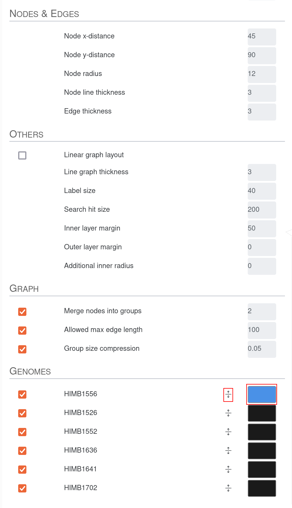
We can switch the color of genomes to highlight their tracks in the graph. As an example, here we change the color of HIMB1556 as this genome is the representative of the the Ampluspelagibacter kiloensis group. We also shift the entry to the top. That way all edges and nodes present in this genome will be colored and also overlay all the other colors. Since a line can only have one color, the coloring is done according to the hierarchy of the genomes.
We could also reduce the compression of the groups to show 20% of the original size instead of 5% to estimate the impact of conserved regions better.

Another usecase might be first linearize the pangenome graph and then tracking the position change of rearranged gene clusters (shown as light green colored nodes).
When we zoom in to that region we can also click on the nodes and check which gene calls are included here.
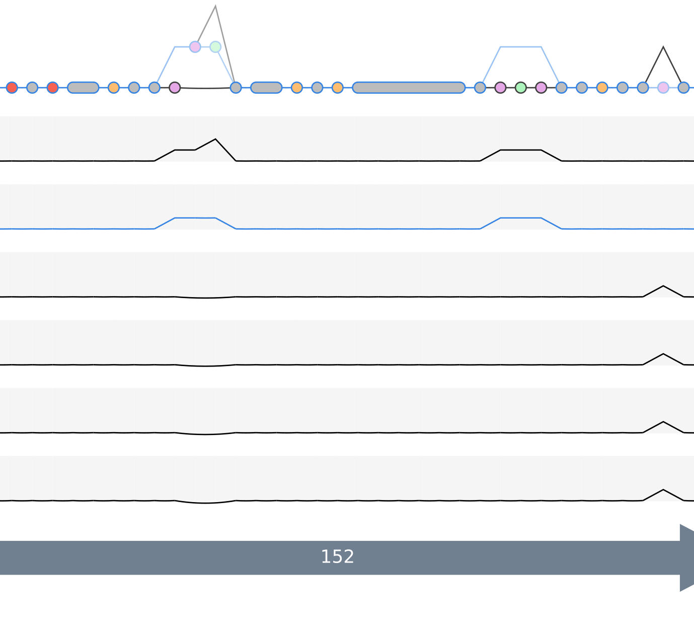
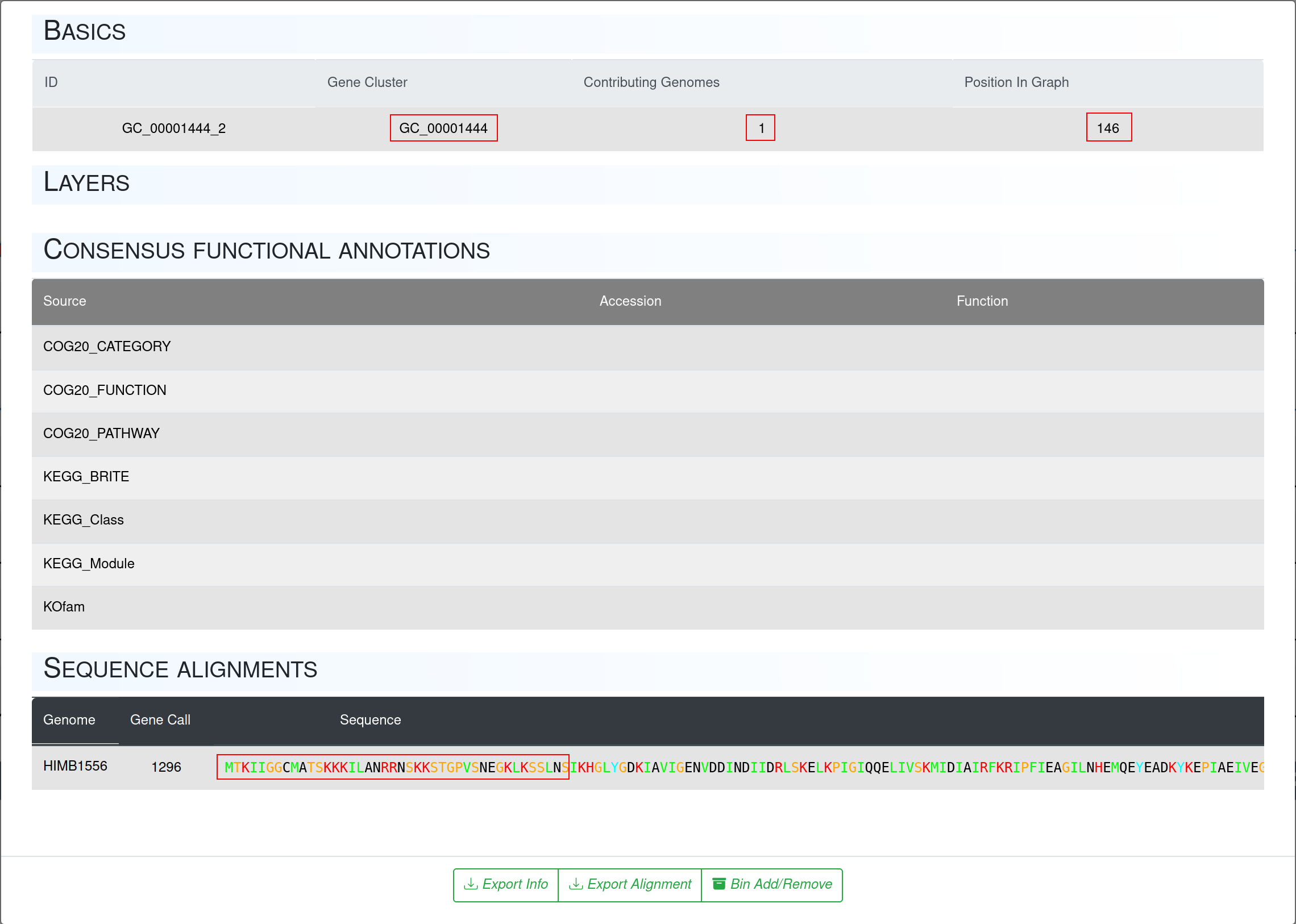

In this case we learn, that gene cluster GC_00001444 not only changed position but in the progress of changing the position the amino acid sequence also slightly changed, visible in the gaps in the beginning in comparison to the second graphic showing no gaps in the same region.