Scaling up your analysis with workflows

Table of Contents
- Getting the data
- Part I: Workflows with anvi’o
- Part II: Pangenomics
- Get publicly available genomes
- Getting genomes ready for the workflow
- Setting up the config file
- Running the pangenomics workflow
- Inspect the pangenome
- Part III: Metagenomics read recruitment
- Conclusion
In this tutorial, you will learn how to contextualize a genome using publicly available data and leverage anvi’o snakemake workflows to upscale your analysis.
This hands-on tutorial is divided into three major sections:
- Introduction to workflows with anvi’o.
- Pangenomics. You will learn how you can obtain publicly available genomes for a given genus/species and run a pangenomics analysis workflow with your genome of interest and the publicly available ones.
- Metagenomics read recruitment. How to download and use publicly available metagenomes and perform read recruitment analysis on your genome of interest or more!
This tutorial was made with anvio v8.
Show/Hide A faster version of this tutorial
If you are following this tutorial and you fall into one of these categories:
- You are taking part in a workshop
- You have a small computer (4 cores) with limited disk space
- You want to complete the tutorial in a short time
Then you should follow the special instructions in these Show/Hide sections.
The rest of the code was all run on a laptop and takes quite a while. You could also use a high performance computer cluster to speed things up.
Getting the data
In this tutorial, we will be using a Prochlorococcus genome as our reference. You should be able to replace it with your favorite genome and see what you can learn from it!
This genome comes from a collection of single-cell assembled genomes by Kashtan et al.. Here is the NCBI webpage for the genome used in this tutorial.
To download the data you will need for this tutorial, copy and paste the following commands in the directory of your choice:
curl -L https://cloud.uol.de/public.php/dav/files/9eHngByzx4L63aq \
     -o WORKFLOW_MATERIAL.tar.gz
tar -xvf WORKFLOW_MATERIAL.tar.gz && cd WORKFLOW_MATERIAL/
Part I: Workflows with anvi’o
In this first part we will create a contigs database for our Prochlorococcus genome. We also want to run some routine commands like anvi-run-hmms to get completion/redundancy estimates, anvi-run-scg-taxonomy to confirm the taxonomic assignment and anvi-run-ncbi-cogs to get some functional annotations.
If you are familiar with anvi’o, you probably have run these commands many times. It gets quite repetitive after a while, and as a good computer scientist you are also lazy. Understandably so. Anvi’o uses snakemake to create multiple workflows for automating commonly-run analyses.
There is an existing blog post made by Alon Shaiber and Meren about snakemake workflows in anvi’o. This part of the tutorial is quite similar to the blog post. The purpose of workflows are (1) to streamline repetitive steps, (2) to improve reproducibility and (3) to enable scalability.
You can use the built-in snakemake workflows in anvi’o with anvi-run-workflow. First, you can ask the program to list the available workflows:
$ anvi-run-workflow --list-workflows

WARNING
===============================================
If you publish results from this workflow, please do not forget to cite
snakemake (doi:10.1093/bioinformatics/bts480)

HMM profiles .................................: 9 sources have been loaded: Bacteria_71 (71 genes, domain: bacteria), Archaea_76 (76 genes, domain: archaea), Ribosomal_RNA_23S (2 genes, domain: None),
                                                Ribosomal_RNA_28S (1 genes, domain: None), Ribosomal_RNA_5S (5 genes, domain: None), Ribosomal_RNA_16S (3 genes, domain: None), Ribosomal_RNA_12S (1 genes, domain:
                                                None), Protista_83 (83 genes, domain: eukarya), Ribosomal_RNA_18S (1 genes, domain: None)
Available workflows ..........................: contigs, metagenomics, pangenomics, phylogenomics, trnaseq, ecophylo, sra_download
config.json
Once you know which workflow you want to use, you need an associated configuration file which allows you to tune each parameters, choose which steps to run and more. You can write this file from scratch, but you can also get a default version with the flag --get-default-config:
anvi-run-workflow -w WORKFLOW-NAME \
                  --get-default-config CONFIG-FILE-NAME
This config file is in JSON format and contains three types of information:
- General workflow parameters like the name of the project, workflow type and version.
- Rule-specific parameters. Basically, for every program used in the workflow you can choose and change parameters, just like if you were to run these programs yourself.
- Output directory names.
Common input files
Most workflows require input files. For example, to run the contigs workflow, you will need a fasta-txt file, which is a file that contains the name and path to FASTA files:
| name | path |
|---|---|
| A_NICE_NAME | /absolute/path/fasta_01.fa |
| ANOTHER_NAME | relative/path/fasta_02.fa.gz |
Another example is the samples-txt file, which contains the paths to metagenomic short read files in a three-column format:
| sample | r1 | r2 |
| sample_01 | sample-01-R1.fastq.gz | sample-01-R2.fastq.gz |
| sample_02 | sample-02-R1.fastq.gz | sample-02-R2.fastq.gz |
Contigs workflow
Go in the first working directory called 01_CONTIGS:
cd 01_CONTIGS
In this directory, you will find two files: a fasta file of a genome, and a fasta-txt which contains the name and path to the fasta file:
$ cat fasta.txt
name	path
Prochlorococcus_JFLQ01	GCF_000634795.1.fasta
Here we are going to use the contigs workflow with our Prochlorococcus genome. First let’s get the default config file for this workflow:
anvi-run-workflow -w contigs \
                  --get-default-config config.json
Have a look at the config.json file. You will see an extensive list of programs and parameters that you can turn ON/OFF and tune.
We don’t need everything, so let’s streamline this file with just what we need. It should look like this:
{
    "fasta_txt": "fasta.txt",
    "anvi_gen_contigs_database": {
        "threads": 2
    },
    "anvi_run_hmms": {
        "run": true,
        "threads": 2,
        "--also-scan-trnas": true
    },
    "anvi_run_kegg_kofams": {
        "run": false
    },
    "anvi_run_ncbi_cogs": {
        "run": true,
        "threads": 2
    },
    "anvi_run_scg_taxonomy": {
        "run": true,
        "threads": 2
    },
    "anvi_script_reformat_fasta": {
        "run": true,
        "--simplify-names": true
    },
    "output_dirs": {
        "FASTA_DIR": "01_FASTA",
        "CONTIGS_DIR": "02_CONTIGS",
        "LOGS_DIR": "00_LOGS"
    },
    "max_threads": 4,
    "config_version": "3",
    "workflow_name": "contigs"
}
Copy the config file Go ahead and modify the config file yourself. For the rest of the tutorial, you can also copy a pre-formatted config file into your working directory:
cp ../00_FILES/config_contigs.json config.json
Before running the workflow, you should have a look at the steps that will be run. For that, you can ask the program to generate a workflow graph:
anvi-run-workflow -w contigs \
                  -c config.json \
                  --save-workflow-graph
If the program cannot generate the pdf file, you need to install graphviz: conda install -y -c anaconda graphviz
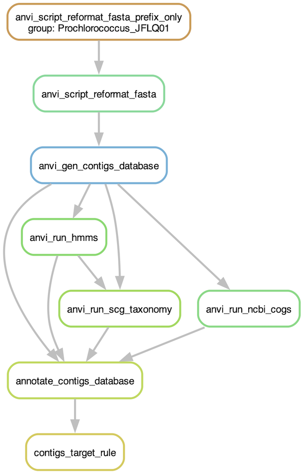
Graph of the contigs workflow
You can also do a “dry run”. The program will display all the jobs that need to be run. Convenient when the workflow graph is too large, or when you work on a remote server:
anvi-run-workflow -w contigs \
                  -c config.json \
                  -A -n -q
If you are happy with what you see, then you can run the actual workflow. It will be rather fast as there is only one genome to process. But you can add as many genomes in the fasta-txt file as you like.
anvi-run-workflow -w contigs \
                  -c config.json
Congratulations, you now have contigs database for your Prochlorococcus genome, if the workflow finished successfully. If not, I’m sure you are able to figure out what is happening by looking at the error message in your terminal and/or reading the log files generated for each program that was run during the workflow.
What do you do once you have a contigs database? Well, you can start asking questions – like, how complete is this genome? To answer that, you can use the program anvi-estimate-genome-completeness to check the completion/redundancy estimates based on the single-copy core genes (SCGs):
anvi-estimate-genome-completeness -c 02_CONTIGS/Prochlorococcus_JFLQ01-contigs.db
And the output should look like a table. The completion/redundancy estimation are quite good.
Genome in "Prochlorococcus_JFLQ01-contigs.db"
===============================================
+--------------------------------+----------+--------------+----------------+----------------+--------------+----------------+
| bin name                       | domain   |   confidence |   % completion |   % redundancy |   num_splits |   total length |
+================================+==========+==============+================+================+==============+================+
| Prochlorococcus_JFLQ01-contigs | BACTERIA |          0.9 |          92.96 |           1.41 |          224 |        1601052 |
+--------------------------------+----------+--------------+----------------+----------------+--------------+----------------+
What else can you do? Check out the artifact page for the contigs-db to get an idea of the programs that use contigs databases.
Part II: Pangenomics
In this part, we will do some comparative genomics using publicly available genomes of Prochlorococcus. You may be interested to do the same with your microorganism of interest, and you should give it a try.
In the case of Prochlorococcus, there are well-described subclades adapted to high-light or low-light environments. Computing a pangenome with multiple Prochlorococcus genomes is one approach we can use to identify in which group our genome belong to, and how similar/unique it is compared to other Prochlorococcus genomes.
Let’s change to a new working directory:
cd ../02_PANGENOMICS
Get publicly available genomes
To download publicly available genome, we can use the program ncbi-genome-download. The following section resembles a previous post written by Alon Shaiber and Meren (AGAIN!?), you can read it here.
You will need to install the program in your anvi’o environment:
pip install ncbi-genome-download
Using ncbi-genome-download This program has many parameters and you should check them all in the help menu:
ncbi-genome-download -h
There are multiple ways to search for specific genomes:
- by using a genus or species name
- by using NCBI taxonomic IDs
- by using an assembly accession number
You can actually provide a list of names/IDs/accessions if you want to download genomes from multiple genera/species.
You can also choose the assembly quality level; for instance, you can request only complete genomes with --assembly-level chromosome,complete, or ask for contigs with --assembly-level contigs.
This program downloads genomes from two possible sources: GenBank or RefSeq (by default). This means it will catch whatever genomes with a given taxonomic assignment in these databases. This is not a fool-proof solution to find all publicly available genomes for a genus/species, but it can probably get you close.
We want to get genomes from NCBI RefSeq, and only the complete genomes. The program will download the genome in genbank format (gbff) and we will ask for a metadata table which contains all the information associated with each genome, like the assembly, BioProject and BioSample accessions. We will search for any genome fitting our criteria with the genus name “Prochlorococcus”:
ncbi-genome-download bacteria \
                     --assembly-level chromosome,complete \
                     --genera "Prochlorococcus" \
                     --metadata metadata.txt
Getting genomes ready for the workflow
Nice, but anvi’o does not work with GenBank format directly. So you can use the following program to create a fasta file for each genome, and also create a fasta-txt which is going to be the input for a pangenomics workflow. By default, this program also extracts the gene calls and functional annotations, if present. So if you want, you can use them and skip gene calling and functional annotation in the upcoming workflow. But at this point, we don’t know how the gene calling and functional annotation were done and for consistency, we will exclude them.
anvi-script-process-genbank-metadata -m metadata.txt \
                                     -o NCBI_genomes \
                                     --output-fasta-txt fasta.txt \
                                     --exclude-gene-calls-from-fasta-txt
Great! We are almost ready for the pangenomics workflow, but we are missing one genome in the fasta-txt. Our genome!
Open the fasta.txt file and add a new line with the name of our Prochlorococcus genome and the path to its fasta file. Your fasta-txt should look more or less like this (either absolute or relative paths are ok). Notice how I renamed the genome to the shortest unique identifier? It will look a lot nicer in the final figure:
name	path
AS9601	NCBI_genomes/Prochlorococcus_marinus_str__AS9601_GCF_000015645_1-contigs.fa
MIT_0912	NCBI_genomes/Prochlorococcus_marinus_str__MIT_0912_GCF_027359595_1-contigs.fa
MIT_0913	NCBI_genomes/Prochlorococcus_marinus_str__MIT_0913_GCF_027359525_1-contigs.fa
MIT_0915	NCBI_genomes/Prochlorococcus_marinus_str__MIT_0915_GCF_027359475_1-contigs.fa
MIT_0917	NCBI_genomes/Prochlorococcus_marinus_str__MIT_0917_GCF_027359575_1-contigs.fa
MIT_0918	NCBI_genomes/Prochlorococcus_marinus_str__MIT_0918_GCF_027359415_1-contigs.fa
MIT_0919	NCBI_genomes/Prochlorococcus_marinus_str__MIT_0919_GCF_027359375_1-contigs.fa
MIT_1013	NCBI_genomes/Prochlorococcus_marinus_str__MIT_1013_GCF_027359395_1-contigs.fa
MIT_1214	NCBI_genomes/Prochlorococcus_marinus_str__MIT_1214_GCF_027359355_1-contigs.fa
MIT_9211	NCBI_genomes/Prochlorococcus_marinus_str__MIT_9211_GCF_000018585_1-contigs.fa
MIT_9215	NCBI_genomes/Prochlorococcus_marinus_str__MIT_9215_GCF_000018065_1-contigs.fa
MIT_9301	NCBI_genomes/Prochlorococcus_marinus_str__MIT_9301_GCF_000015965_1-contigs.fa
MIT_9303	NCBI_genomes/Prochlorococcus_marinus_str__MIT_9303_GCF_000015705_1-contigs.fa
MIT_9312	NCBI_genomes/Prochlorococcus_marinus_str__MIT_9312_GCF_000012645_1-contigs.fa
MIT_9313	NCBI_genomes/Prochlorococcus_marinus_str__MIT_9313_GCF_000011485_1-contigs.fa
MIT_9515	NCBI_genomes/Prochlorococcus_marinus_str__MIT_9515_GCF_000015665_1-contigs.fa
NATL1A	NCBI_genomes/Prochlorococcus_marinus_str__NATL1A_GCF_000015685_1-contigs.fa
NATL2A	NCBI_genomes/Prochlorococcus_marinus_str__NATL2A_GCF_000012465_1-contigs.fa
CCMP1375	NCBI_genomes/Prochlorococcus_marinus_subsp__marinus_str__CCMP1375_GCF_000007925_1-contigs.fa
CCMP1986	NCBI_genomes/Prochlorococcus_marinus_subsp__pastoris_str__CCMP1986_GCF_000011465_1-contigs.fa
MIT_0604	NCBI_genomes/Prochlorococcus_sp__MIT_0604_GCF_000757845_1-contigs.fa
MIT_0801	NCBI_genomes/Prochlorococcus_sp__MIT_0801_GCF_000757865_1-contigs.fa
RS01	NCBI_genomes/Prochlorococcus_sp__RS01_GCF_001989435_1-contigs.fa
RS04	NCBI_genomes/Prochlorococcus_sp__RS04_GCF_001989455_1-contigs.fa
RS50	NCBI_genomes/Prochlorococcus_sp__RS50_GCF_001989415_1-contigs.fa
Prochlororcoccus_JFLQ01	../01_CONTIGS/GCF_000634795.1.fasta
Copy the fasta.txt file You can modify the fasta.txt to your liking, but for the rest of the tutorial, you can also copy the above fasta.txt into your working directory:
cp ../00_FILES/fasta_pangenomics.txt fasta.txt
Show/Hide Get a smaller list of genomes
If you are following the faster version of this tutorial, you can copy a different fasta.txt file which only contains 9 of the 26 genomes that were downloaded:
cp ../00_FILES/fasta_pangenomics_fast.txt fasta.txt
Setting up the config file
We have the main input for the pangenomics workflow. Next, we need a config file. Again, we can write the config file ourselves, or we can get the default one for the pangenomics workflow and modify it for our needs.
anvi-run-workflow -w pangenomics \
                  --get-default-config config.json
Here is the modified version of the config file. With this config file, we will create contigs databases for each genome and annotate their genes with NCBI COGs and KEGG. In addition to the mandatory steps of a pangenomics analysis, we will compute the average nucleotide identity (ANI) between all genomes with anvi-compute-genome-similarity. We will be able to display the ANI heatmap in the interactive interface later.
{
    "fasta_txt": "fasta.txt",
    "anvi_gen_contigs_database": {
        "threads": 2
    },
    "anvi_run_hmms": {
        "run": true,
        "threads": 2
    },
    "anvi_run_kegg_kofams": {
        "run": true,
        "threads": 2
    },
    "anvi_run_ncbi_cogs": {
        "run": true,
        "threads": 2
    },
    "anvi_run_scg_taxonomy": {
        "run": true,
        "threads": 2
    },
    "anvi_script_reformat_fasta": {
        "run": true,
        "--simplify-names": true
    },
    "anvi_pan_genome": {
        "threads": 4
    },
    "anvi_compute_genome_similarity": {
        "run": true,
        "threads": 4
    },
    "project_name": "Prochlorococcus",
    "external_genomes": "external-genomes.txt",
    "output_dirs": {
        "FASTA_DIR": "01_FASTA",
        "CONTIGS_DIR": "02_CONTIGS",
        "PAN_DIR": "03_PAN",
        "LOGS_DIR": "00_LOGS"
    },
    "max_threads": 4,
    "config_version": "3",
    "workflow_name": "pangenomics"
}
Copy the config file You can modify the config file to your liking, but for the rest of the tutorial, you can also copy the above version into your working directory:
cp ../00_FILES/config_pangenomics.json config.json
If you know what you are doing, you can change the number of threads for each job in the config.json. And also the max number of threads, at the end of the config file.
Show/Hide Modify the config file
Some steps will take a lot of time – like gene functional annotation with KEGG, or computing the average nucleotide identity. The latter is optional, but very interesting. For the sake of time, you can use this config file which skips KEGG annotation, and SCG taxonomy assignment.
{
    "fasta_txt": "fasta.txt",
    "anvi_gen_contigs_database": {
        "threads": 2
    },
    "anvi_run_hmms": {
        "run": true,
        "threads": 2
    },
    "anvi_run_kegg_kofams": {
        "run": false
    },
    "anvi_run_ncbi_cogs": {
        "run": true,
        "threads": 2
    },
    "anvi_run_scg_taxonomy": {
        "run": false
    },
    "anvi_script_reformat_fasta": {
        "run": true,
        "--simplify-names": true
    },
    "anvi_pan_genome": {
        "threads": 4
    },
    "anvi_compute_genome_similarity": {
        "run": true,
        "threads": 4
    },
    "project_name": "Prochlorococcus",
    "external_genomes": "external-genomes.txt",
    "output_dirs": {
        "FASTA_DIR": "01_FASTA",
        "CONTIGS_DIR": "02_CONTIGS",
        "PAN_DIR": "03_PAN",
        "LOGS_DIR": "00_LOGS"
    },
    "max_threads": 4,
    "config_version": "3",
    "workflow_name": "pangenomics"
}
You can copy that config file from the datapack:
cp ../00_FILES/config_pangenomics_fast.json config.json
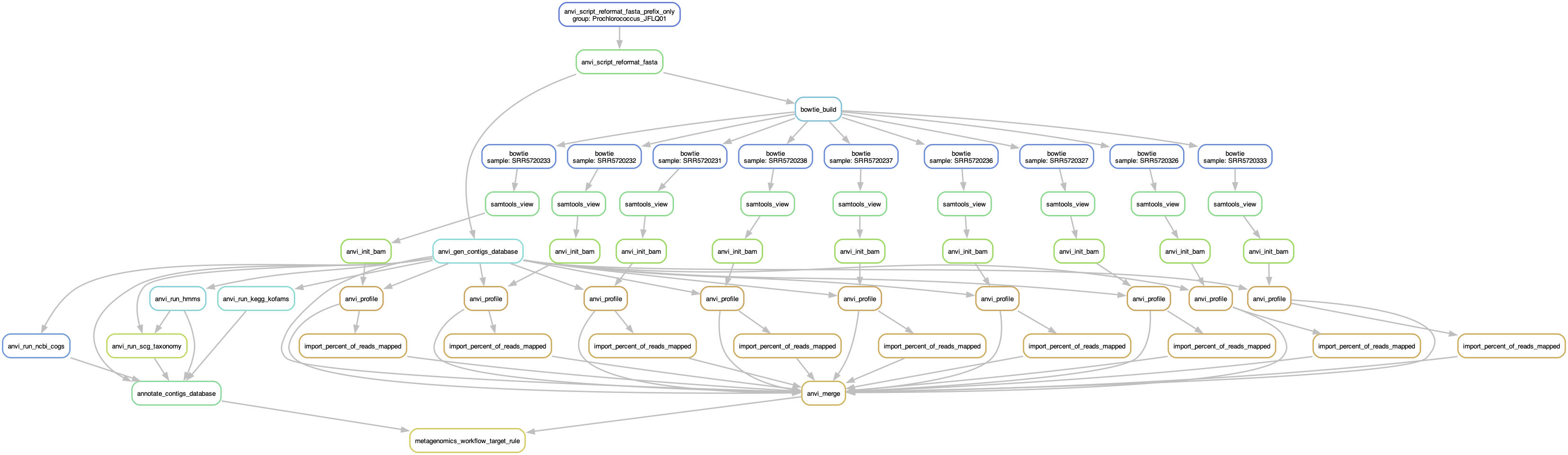
Before running the workflow, you should look at the workflow graph and make sure everything will go as planned:
anvi-run-workflow -w pangenomics \
                  -c config.json \
                  --save-workflow-graph
And yes, that is the output. A rather wide figure, but if you zoom in you will see all the steps planned for each genome. Eventually, all steps funnel into the programs anvi-pan-genome and anvi-compute-genome-similarity.

Graph of the pangenomics workflow
Already have contigs databases? What if you already have contigs dbs for all of your genomes? Well, you can skip the first step of the pangenomics workflow by using an external-genomes-txt, which is simply a table with the name and path to each contigs database. If the “external_genomes” entry in your config file matches the file name of your external-genomes-txt, then the workflow will only start from there, assuming previous steps were completed.
Running the pangenomics workflow
If you feel confident about your config file, let’s run the workflow:
anvi-run-workflow -w pangenomics \
                  -c config.json
Have a break while the workflow is running (~5-10 minutes).
Roses are red. Violets are blue. Computer goes BEEP BOOP. More time for you.
Inspect the pangenome
We can use anvi-display-pan to open an interactive interface and investigate our pangenome:
anvi-display-pan -g 03_PAN/Prochlorococcus-GENOMES.db \
                 -p 03_PAN/Prochlorococcus-PAN.db
After a few modifications on the interface, you should be able to see something like this:
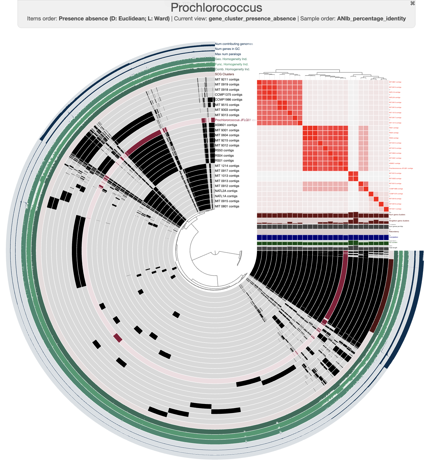
Prochlorococcus pangenome
We can see that our genome clusters quite nicely with a group of genomes. For instance, it is closely related to the genome called AS9601, which is part of the high-light group II (Kettler et al. 2007, Biller et al. 2014, Delmont and Eren, 2018).
Good job! You have learned how to rapidly get genomes of a given taxonomy and leverage the pangenomics workflow in anvi’o. Now go back to the beginning of this section and start again with your favorite taxon 🎉
Part III: Metagenomics read recruitment
In this part of the tutorial, we want to find relevant metagenomes and perform read-recruitment on our Prochlorococcus genome.
Find and download metagenomes
Show/Hide What if you don't want to download metagenomes?
Just skip this part. Smaller version of these metagenomes are available in the datapack, and you will find instructions to use them later.
Resources to get metagenomes
If you want to download publicly available metagenomes, there are multiple resources. The following list is not exhaustive and we would love to hear about your favorite ones. We have been discussing them on anvi’o discord and you are welcome to join and share with the community.
-
If you have a BioProject accession (like PRJNA385855), you can use NCBI and their SRA run selector or MGnify. Both of these websites will allow you to download a list of accessions that we will use later in the tutorial.
-
If you want samples based on their characteristics, either biological (sample type) or technical (number of reads) you can use the following websites: GMrepo for human gut samples, MarineMetagenomeDB for marine samples and TerrestrialMetagenomeDB for soil samples.
-
Alternatively, you can use sandpiper to search for metagenomes where a taxon is detected. Another powerful resource is branchwater: you can upload your own genome and search for metagneomes in which it occurs!
-
And sometimes, you can find SRA accession numbers directly from a publication, likely in supplementary data.
In the end, you will need a list of SRA accession numbers for each sample. It should look like SRR#### or ERR#### (look for the double R).
First step is to go to a new working directory:
cd ../03_SRA_DOWNLOAD/
List of SRA accessions
For this example, we will download some metagenomes from the Bermuda Atlantic Time-series Study (BATS). I found the following accession numbers from a paper by Biller et al. 2018. The samples are coming from three sampling dates, and three depths.
| Accession | Date | Depth |
|---|---|---|
| SRR5720233 | 21.02.03 | 1 |
| SRR5720232 | 21.02.03 | 40 |
| SRR5720231 | 21.02.03 | 180 |
| SRR5720238 | 22.03.03 | 1 |
| SRR5720237 | 22.03.03 | 80 |
| SRR5720236 | 22.03.03 | 180 |
| SRR5720327 | 22.04.03 | 10 |
| SRR5720326 | 22.04.03 | 80 |
| SRR5720333 | 22.04.03 | 180 |
The accession numbers can be found in SRA_accession_list.txt:
$ cat SRA_accession_list.txt
SRR5720233
SRR5720232
SRR5720231
SRR5720238
SRR5720237
SRR5720236
SRR5720327
SRR5720326
SRR5720333
Setting up the config file
To download these metagenomes, we will use another workflow from anvi-run-workflow: SRA download. And like for the previous workflows, we will need a config file as well as a required input file, which is the SRA_accession_list.txt. Let’s get the default config file:
anvi-run-workflow -w sra_download \
                  --get-default-config config.json
There are three steps in this workflow, all mandatory. We can adjust the default number of threads for each steps:
{
    "SRA_accession_list": "SRA_accession_list.txt",
    "prefetch": {
        "--max-size": "40g",
        "threads": 2
    },
    "fasterq_dump": {
        "threads": 2
    },
    "pigz": {
        "threads": 2
    },
    "output_dirs": {
        "SRA_prefetch": "01_NCBI_SRA",
        "FASTAS": "02_FASTQ",
        "LOGS_DIR": "00_LOGS"
    },
    "max_threads": 4,
    "config_version": "3",
    "workflow_name": "sra_download"
}
Copy the config file A copy of this config file is available for you:
cp ../00_FILES/config_sra_download.json config.json
Download the metagenomes
The total size of these metagenomes is 46 Gb when compressed. With the temporary files, it can use a large amount of disk space. Make sure you have enough space, then run the workflow.
anvi-run-workflow -w sra_download \
                  -c config.json
If everything went well, you should have the metagenomes and a samples-txt. And that is very good news because that file is the required input file for the upcoming metagenomics workflow.
The metagenomics workflow
This workflow has many components and can be used in different “modes”. For instance, you could provide a list of metagenomes in a samples-txt file and the workflow will take care of the assembly, read recruitment, creation of the contigs database and profile database, and once it is done you will be ready for binning. Another mode, referred to as “reference mode”, can be used when you want to recruit reads from metagenomes (also called mapping) on a reference sequence. That reference can be any fasta file, like a genome, multiple genomes or an assembly. At the end, you will also get a contigs database and a profile database.
The workflows can include third party software like assemblers. Make sure you have the right software installed in the anvi’o environment before running the workflow.
In this tutorial, we will follow the “reference mode” and recruit reads from the metagenomes that we downloaded to our Prochlorococcus genome. For more information about everything you can do with this workflow, go check the associated help page.
Now we can move into the new working directory:
cd ../04_READ_RECRUITMENT
Setting up the config file
Like any workflow in anvi’o, we need a config file. You can get the default file by running this command:
anvi-run-workflow -w metagenomics \
                  --get-default-config config.json
It includes many steps that are only used in the mode when you want to perform assembly. Here is a config file with just the steps we need for “reference mode”, using a maximum of 4 threads (feel free to increase the number of threads if your machine can handle it):
{
    "fasta_txt": "fasta.txt",
    "anvi_gen_contigs_database": {
        "--project-name": "{group}",
        "threads": 2
    },
    "anvi_run_hmms": {
        "run": true,
        "threads": 5,
        "--also-scan-trnas": true
    },
    "anvi_run_kegg_kofams": {
        "run": true,
        "threads": 4
    },
    "anvi_run_ncbi_cogs": {
        "run": true,
        "threads": 5
    },
    "anvi_run_scg_taxonomy": {
        "run": true,
        "threads": 6
    },
    "anvi_script_reformat_fasta": {
        "run": true,
        "--prefix": "{group}",
        "--simplify-names": true
    },
    "samples_txt": "samples.txt",
    "bowtie": {
        "additional_params": "--no-unal",
        "threads": 4
    },
    "anvi_profile": {
        "threads": 4,
        "--sample-name": "{sample}"
    },
    "anvi_merge": {
        "--sample-name": "{group}",
        "threads": 4
    },
    "references_mode": true,
    "output_dirs": {
        "FASTA_DIR": "01_FASTA",
        "CONTIGS_DIR": "02_CONTIGS",
        "MAPPING_DIR": "03_MAPPING",
        "PROFILE_DIR": "04_ANVIO_PROFILE",
        "MERGE_DIR": "05_MERGED",
        "LOGS_DIR": "00_LOGS"
    },
    "max_threads": 4,
    "config_version": "3",
    "workflow_name": "metagenomics"
}
Copy the config file You can copy the above config file into your working directory:
cp ../00_FILES/config_metagenomics.json config.json
Show/Hide Another config file
To make this workflow faster, we can skip a few steps like the KEGG annotation and the taxonomy estimation:
{
    "fasta_txt": "fasta.txt",
    "anvi_gen_contigs_database": {
        "--project-name": "{group}",
        "threads": 2
    },
    "anvi_run_hmms": {
        "run": true,
        "threads": 4,
        "--also-scan-trnas": true
    },
    "anvi_run_kegg_kofams": {
        "run": false
    },
    "anvi_run_ncbi_cogs": {
        "run": true,
        "threads": 4
    },
    "anvi_run_scg_taxonomy": {
        "run": false
    },
    "anvi_script_reformat_fasta": {
        "run": true,
        "--prefix": "{group}",
        "--simplify-names": true
    },
    "samples_txt": "samples.txt",
    "bowtie": {
        "additional_params": "--no-unal",
        "threads": 4
    },
    "anvi_profile": {
        "threads": 4,
        "--sample-name": "{sample}"
    },
    "anvi_merge": {
        "--sample-name": "{group}",
        "threads": 4
    },
    "references_mode": true,
    "output_dirs": {
        "FASTA_DIR": "01_FASTA",
        "CONTIGS_DIR": "02_CONTIGS",
        "MAPPING_DIR": "03_MAPPING",
        "PROFILE_DIR": "04_ANVIO_PROFILE",
        "MERGE_DIR": "05_MERGED",
        "LOGS_DIR": "00_LOGS"
    },
    "max_threads": 4,
    "config_version": "3",
    "workflow_name": "metagenomics"
}
You can copy that config file into your working directory:
cp ../00_FILES/config_metagenomics_fast.json config.json
Getting the required files
There are two files required for this workflow, in addition to the config file. The first one is a fasta-txt, and it is already present in the working directory.
$ cat fasta.txt
name	path
Prochlorococcus_JFLQ01	../01_CONTIGS/GCF_000634795.1.fasta
The second file is a samples-txt file. If you followed the previous part and downloaded the metagenomes using the SRA download workflow, then a samples.txt was created and you can copy it to your current working directory:
cp ../03_SRA_DOWNLOAD/samples.txt .
If you skipped the previous part, a smaller set of these metagenomes is included in the datapack in the directory 00_SAMPLES and you can copy this samples-txt file into your working directory:
cp ../00_FILES/samples.txt .
Generate the workflow graph
Like we did for the other workflows, it is always a good idea to generate the workflow graph (or do a dry run) and make sure the workflow includes all the steps that you expect:
anvi-run-workflow -w metagenomics \
                  -c config.json \
                  --save-workflow-graph
Read recruitment workflow graph
Run the workflow
If you are happy about what you see in the workflow graph, then you can run the workflow:
anvi-run-workflow -w metagenomics \
                  -c config.json
Start an interactive interface
Before opening the interactive interface, we can add some information about each sample. In the file additional_layers.txt, you will find information about the sampling date and depth:
$ cat additional_layers.txt
Accession	Date	Depth
SRR5720233	21.02.03	1
SRR5720232	21.02.03	40
SRR5720231	21.02.03	180
SRR5720238	22.03.03	1
SRR5720237	22.03.03	80
SRR5720236	22.03.03	180
SRR5720327	22.04.03	10
SRR5720326	22.04.03	80
SRR5720333	22.04.03	180
And you can use anvi-import-misc-data to add that information to the profile database:
anvi-import-misc-data -p 05_MERGED/Prochlorococcus_JFLQ01/PROFILE.db \
                      -t layers \
                      additional_layers.txt
Then start the interactive interface:
anvi-interactive -c 02_CONTIGS/Prochlorococcus_JFLQ01-contigs.db \
                 -p 05_MERGED/Prochlorococcus_JFLQ01/PROFILE.db
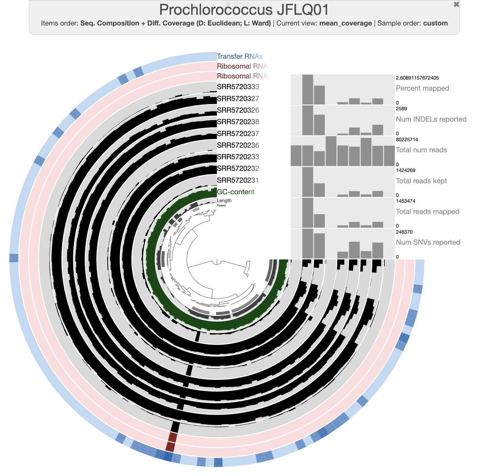
Interactive interface
By default, the interactive interface will display the (log transformed) mean coverage of each split. The following figure displays detection (non-transformed) and the scale for each sample is from 0 to 1. After a little bit of prettification, you can improve the figure.
If you don’t want to spend your precious time making modifications on the interactive interface, you can import the state file present in the directory. Then you should be able to select the state “detection” when clicking the “load state” button on the interactive interface.
anvi-import-state -p 05_MERGED/Prochlorococcus_JFLQ01/PROFILE.db \
                  -s state.json \
                  -n detection
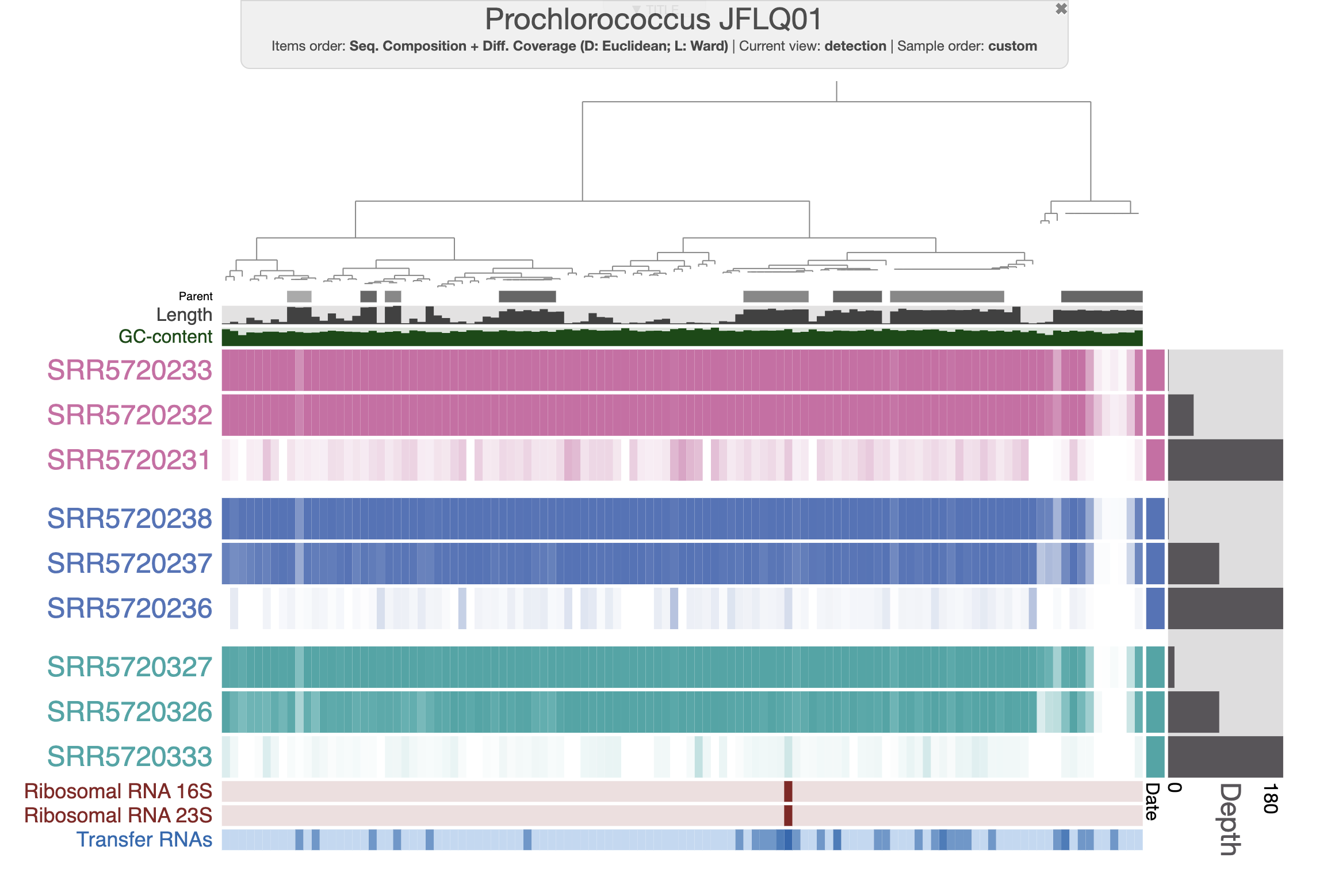
Interactive interface
With the figure above, you can clearly see the distribution of that Prochlorococcus population in the first two depths for each time point. And you can also notice the absence of detection for a fraction of the genome. Well, that’s simply because the genome we are using doesn’t represent the local population, yet they are close enough to allow read recruitment. You can inspect random splits and look at the amount of SNVs to understand how different are your genome and the population occurring in the Bermuda sea at the time.
Using multiple genomes for read recruitment Recruiting reads from metagenomes onto a single genome will create a lot of non-specific mapping: reads that come from another population but can still partially align to your reference genome. To improve the last part of this tutorial, you could consider putting together multiple genomes of Prochlorococcus and performing competitive mapping by concatenating all genomes in a single fasta file. This way, during the mapping, the short reads would map to the best matching genome in the set. If you are familiar with anvi’o, you may recognize that this is the first step to generating a metapangenome.
Conclusion
This tutorial exists to showcase the scalability of anvi’o workflows and how you can leverage publicly available genomes and metagenomes to investigate your scientific questions. If you have comments and questions, feel free to reach out to us and the community on Discord. Thanks for reading!