Visualizing mass spec data with anvi'o

Table of Contents
- Introduction to the Project and Original Data
- The primary data for anvi’o analysis and visualization
- Visualizing molecular formula across microbial consortia
- Adding additional data layers for ‘items’ (molecular formula)
- Adding additional data layers for ‘layers’ (samples)
- Fine-tuning the display aesthetics for better structure and clarity
- Conclusion
This is a tutorial to explain how the anvi’o interactive interface can be used to visualize FT-ICR-MS data that relies upon a real-world dataset. Some parts of the tutorial will be very specific to the dataset investigated for the particular reserach qeustion here, but once the input data is ready in an anvi’o compatible form, it will be much easeir for anyone to recognize how their data could also fit into that form.
This tutorial is tailored for anvi’o v8 but will probably work for later versions as well (perhaps with minor command modifications). You can learn the version of your installation by running anvi-interactive -v in your terminal.
Introduction to the Project and Original Data
As part of a recent project with Sinikka Lennartz and Carina Bunse, I was interested in investigating how microbial interactions influence the composition of dissolved organic matter (DOM).
To do this, we selected four bacterial isolates originating from the same North Sea water sample and grew them in a full factorial setup. We grew isolates in every possible combination, ranging from individual strains all by themselves to two-, three-, and one four-member consortia, as shown here:
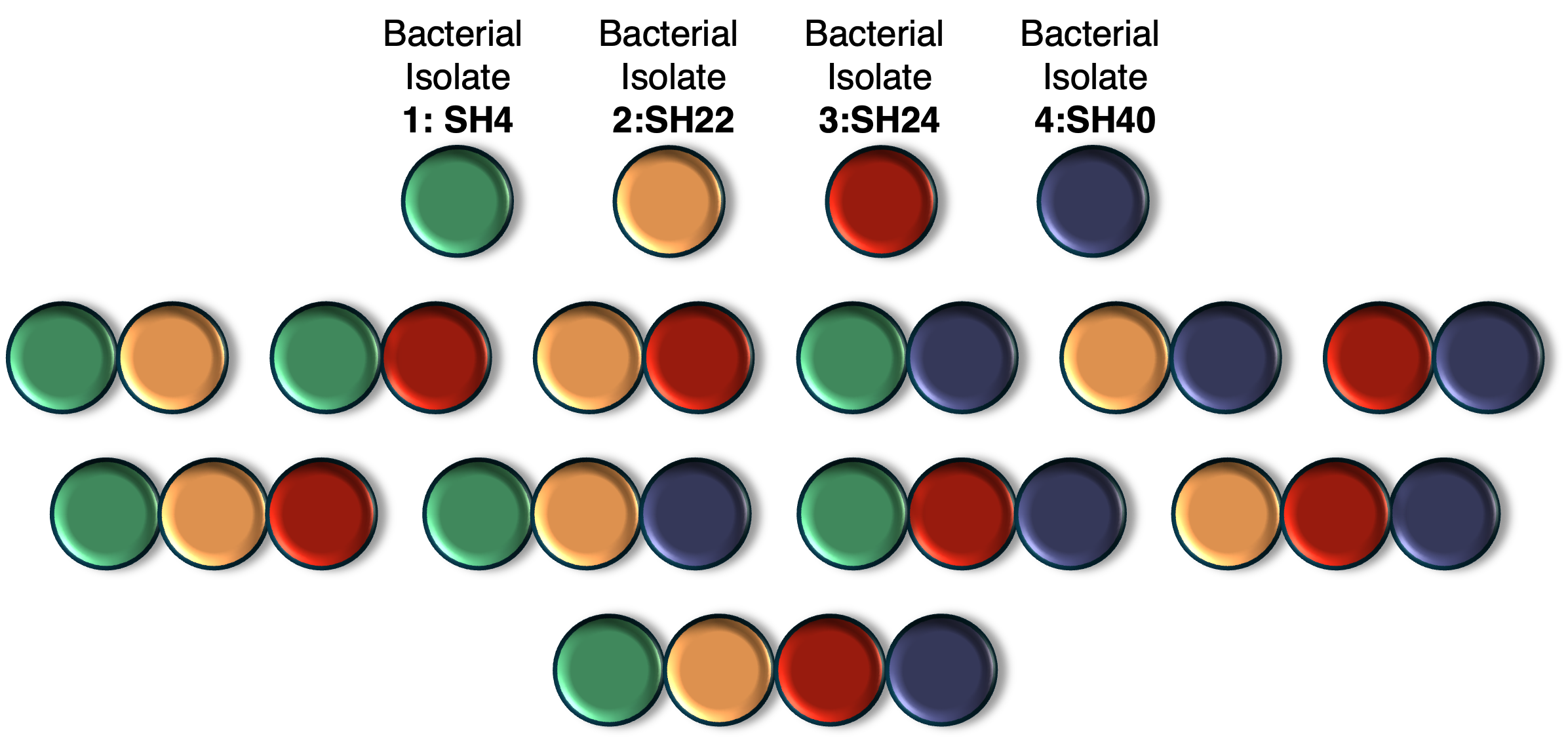
Full factorial setup of four bacterial isolates, all belonging to the Roseobacter clade. We are using the identifiers given to them by Sarah Hahnke, who originally isolated these strains—which is why they are called SH :)
We knew that each of these strains grew well in minimal artificial seawater medium, and for our experiment, we provided glucose as the source of carbon and energy. The central idea was to survey the fate of compounds produced by pure cultures in the presence of other bacteria.
Using solid-phase extraction with PPL cartridges, we isolated dissolved organic matter from each culture at approximately mid-exponential phase. Some may refer to this microbially produced DOM as the “exometabolome”, though this term is debated, as many of the compounds we observed do not appear to be associated with microbial metabolism (at least as far as we can currently tell). We also generated medium and cartridge blanks and then measured all samples on the FT-ICR-MS. All measurements took place in the Marine Geochemistry Group at the University of Oldenburg.
The FT-ICR-MS provides highly resolved mass measurements that enable us to assign molecular formulas to each mass with high accuracy. That said, unlike the more common LC-MS/MS measurements, FT-ICR-MS data are one-dimensional. This means we obtain very accurate mass values, but no structural information, and therefore cannot assign precise molecular identities. We used the in-house developed software ICBM-OCEAN to assign molecular formulas to each mass, following a set of predefined rules, which you can learn more about here.
This is what the final output looks like:
| id | mz | diff | reference | formula | formula_isotopefree | formula_ion | homseries | totalc | H.C | O.C | C | H | O | N | S | P | Cl | Na | C13 | O18 | N15 | S34 | Cl37 | Co | Cu.i | Cu.ii | Cu65.i | Cu65.ii | Fe.ii | Fe.iii | Fe54.ii | Fe54.iii | Br79 | Br81 | Ni.ii | Ni60.ii | Zn.ii | Zn66.ii | I | MDL_3 | ResPow | m1 | SE | present_in | AI | AI.mod | DBE | Aromatic | Aromatic.O_rich | Aromatic.O_poor | Highly.unsaturated | Highly.unsaturated.O_rich | Highly.unsaturated.O_poor | Unsaturated | Unsaturated.O_rich | Unsaturated.O_poor | Unsaturated.with.N | Saturated | Saturated.O_rich | Saturated.O_poor | mean_signal_to_MDL | isoratioC13.1 | isoratioC13.2 | isoratio_O18 | isoratioS34 | isoratioN15 | isoratioBr81.1 | isoratioBr81.2 | isoratioCu.i_65 | isoratioCu.ii_65 | isoratioFe.ii_54 | isoratioFe.iii_54 | isoratioZn.ii_66 | isoratioNi.ii_60 | isoratioCl37 | isorat_sdC13.1 | isorat_sdC13.2 | isorat_sd_O18 | isorat_sd_S34 | isorat_sd_N15 | homnetworkmember | diff_filter | alternative_formula | Sample1_masslistsSPE.blank_1.1.18_1_31680.csv | Sample2_masslistsSPE.blank_1.1.18_1_31668.csv | Sample3_masslistsMGC2100451_SL_AMC_Add.on_FT__1.1.4_1_31584.csv | Sample4_masslistsMGC2100451_SL_AMC_Add.on_FT__1.1.4_1_31572.csv | Sample5_masslistsMGC2100450_SL_AMC_Add.on_FT__1.1.10_1_31625.csv | Sample6_masslistsMGC2100450_SL_AMC_Add.on_FT__1.1.10_1_31603.csv | Sample7_masslistsMGC2100449_SL_AMC_Add.on_FT__1.1.15_1_31659.csv | Sample8_masslistsMGC2100449_SL_AMC_Add.on_FT__1.1.15_1_31647.csv | Sample9_masslistsMGC2100448_SL_AMC_Add.on_FT_x05_1.1.42_1_31755.csv | Sample10_masslistsMGC2100448_SL_AMC_Add.on_FT_x05_1.1.42_1_31743.csv | Sample11_masslistsMGC2100447_SL_AMC_Add.on_FT__1.1.12_1_31653.csv | Sample12_masslistsMGC2100447_SL_AMC_Add.on_FT__1.1.12_1_31641.csv | Sample13_masslistsMGC2100446_SL_AMC_Add.on_FT_x05_1.1.33_1_31730.csv | Sample14_masslistsMGC2100446_SL_AMC_Add.on_FT_x05_1.1.33_1_31720.csv | Sample15_masslistsMGC2100445_SL_AMC_Add.on_FT__1.1.16_1_31676.csv | Sample16_masslistsMGC2100445_SL_AMC_Add.on_FT__1.1.16_1_31664.csv | Sample17_masslistsMGC2100444_SL_AMC_Add.on_FT__1.1.13_1_31655.csv | Sample18_masslistsMGC2100444_SL_AMC_Add.on_FT__1.1.13_1_31643.csv | Sample19_masslistsMGC2100443_SL_AMC_Add.on_FT__1.1.6_1_31588.csv | Sample20_masslistsMGC2100443_SL_AMC_Add.on_FT__1.1.6_1_31576.csv | Sample21_masslistsMGC2100442_SL_AMC_Add.on_FT__1.1.17_1_31678.csv | Sample22_masslistsMGC2100442_SL_AMC_Add.on_FT__1.1.17_1_31666.csv | Sample23_masslistsMGC2100441_SL_AMC_Add.on_FT__1.1.7_1_31621.csv | Sample24_masslistsMGC2100441_SL_AMC_Add.on_FT__1.1.7_1_31597.csv | Sample25_masslistsMGC2100440_SL_AMC_Add.on_FT__1.1.3_1_31582.csv | Sample26_masslistsMGC2100440_SL_AMC_Add.on_FT__1.1.3_1_31570.csv | Sample27_masslistsMGC2100439_SL_AMC_Add.on_FT__1.1.14_1_31657.csv | Sample28_masslistsMGC2100439_SL_AMC_Add.on_FT__1.1.14_1_31645.csv | Sample29_masslistsMGC2100438_SL_AMC_Add.on_FT__1.1.9_1_31623.csv | Sample30_masslistsMGC2100438_SL_AMC_Add.on_FT__1.1.9_1_31601.csv | Sample31_masslistsMGC2100437_SL_AMC_Add.on_FT__1.1.11_1_31651.csv | Sample32_masslistsMGC2100437_SL_AMC_Add.on_FT__1.1.11_1_31637.csv | Sample33_masslistsMGC2100436_SL_AMC_Add.on_FT__1.1.5_1_31586.csv | Sample34_masslistsMGC2100436_SL_AMC_Add.on_FT__1.1.5_1_31574.csv | Sample35_masslistsMGC2100435_SL_AMC_Add.on_FT_x05_1.1.24_1_31684.csv | Sample36_masslistsMGC2100435_SL_AMC_Add.on_FT_x05_1.1.24_1_31672.csv | Sample37_masslistsMGC2100434_SL_AMC_Add.on_FT_x05_1.1.26_1_31703.csv | Sample38_masslistsMGC2100434_SL_AMC_Add.on_FT_x05_1.1.26_1_31691.csv | Sample39_masslistsMGC2100433_SL_AMC_Add.on_FT__1.2.24_1_31524.csv | Sample40_masslistsMGC2100433_SL_AMC_Add.on_FT__1.2.24_1_31514.csv | Sample41_masslistsMGC2100432_SL_AMC_Add.on_FT__1.2.20_1_31504.csv | Sample42_masslistsMGC2100432_SL_AMC_Add.on_FT__1.2.20_1_31492.csv | Sample43_masslistsMGC2100431_SL_AMC_Add.on_FT__1.2.16_1_31481.csv | Sample44_masslistsMGC2100431_SL_AMC_Add.on_FT__1.2.16_1_31469.csv | Sample45_masslistsMGC2100430_SL_AMC_Add.on_FT__1.1.4_1_31549.csv | Sample46_masslistsMGC2100430_SL_AMC_Add.on_FT__1.1.4_1_31539.csv | Sample47_masslistsMGC2100429_SL_AMC_Add.on_FT__1.2.27_1_31530.csv | Sample48_masslistsMGC2100429_SL_AMC_Add.on_FT__1.2.27_1_31520.csv | Sample49_masslistsMGC2100428_SL_AMC_Add.on_FT__1.2.23_1_31510.csv | Sample50_masslistsMGC2100428_SL_AMC_Add.on_FT__1.2.23_1_31498.csv | Sample51_masslistsMGC2100427_SL_AMC_Add.on_FT_x05_1.1.30_1_31724.csv | Sample52_masslistsMGC2100427_SL_AMC_Add.on_FT_x05_1.1.30_1_31714.csv | Sample53_masslistsMGC2100426_SL_AMC_Add.on_FT__1.2.15_1_31479.csv | Sample54_masslistsMGC2100426_SL_AMC_Add.on_FT__1.2.15_1_31467.csv | Sample55_masslistsMGC2100425_SL_AMC_Add.on_FT_x08_1.1.21_1_31629.csv | Sample56_masslistsMGC2100425_SL_AMC_Add.on_FT_x08_1.1.21_1_31617.csv | Sample57_masslistsMGC2100425_SL_AMC_Add.on_FT_x05_1.1.22_1_31635.csv | Sample58_masslistsMGC2100425_SL_AMC_Add.on_FT_x05_1.1.22_1_31633.csv | Sample59_masslistsMGC2100423_SL_AMC_Add.on_FT_x05_1.1.35_1_31749.csv | Sample60_masslistsMGC2100423_SL_AMC_Add.on_FT_x05_1.1.35_1_31737.csv | Sample61_masslistsMGC2100422_SL_AMC_Add.on_FT_x05_1.1.38_1_31770.csv | Sample62_masslistsMGC2100422_SL_AMC_Add.on_FT_x05_1.1.38_1_31760.csv | Sample63_masslistsMGC2100421_SL_AMC_Add.on_FT_x05_1.1.19_1_31627.csv | Sample64_masslistsMGC2100421_SL_AMC_Add.on_FT_x05_1.1.19_1_31619.csv | Sample65_masslistsMGC2100420_SL_AMC_Add.on_FT_x05_1.1.34_1_31747.csv | Sample66_masslistsMGC2100420_SL_AMC_Add.on_FT_x05_1.1.34_1_31735.csv | Sample67_masslistsMGC2100419_SL_AMC_Add.on_FT_x05_1.1.41_1_31776.csv | Sample68_masslistsMGC2100419_SL_AMC_Add.on_FT_x05_1.1.41_1_31766.csv | Sample69_masslistsMGC2100418_SL_AMC_Add.on_FT_x05_1.1.32_1_31728.csv | Sample70_masslistsMGC2100418_SL_AMC_Add.on_FT_x05_1.1.32_1_31718.csv | Sample71_masslistsMGC2100417_SL_AMC_Add.on_FT_x05_1.1.36_1_31751.csv | Sample72_masslistsMGC2100417_SL_AMC_Add.on_FT_x05_1.1.36_1_31739.csv | Sample73_masslistsMGC2100416_SL_AMC_Add.on_FT__1.2.17_1_31483.csv | Sample74_masslistsMGC2100416_SL_AMC_Add.on_FT__1.2.17_1_31471.csv | Sample75_masslistsMGC2100415_SL_AMC_Add.on_FT__1.2.8_1_31433.csv | Sample76_masslistsMGC2100415_SL_AMC_Add.on_FT__1.2.8_1_31421.csv | Sample77_masslistsMGC2100414_SL_AMC_Add.on_FT__1.2.3_1_31408.csv | Sample78_masslistsMGC2100414_SL_AMC_Add.on_FT__1.2.3_1_31396.csv | Sample79_masslistsMGC2100413_SL_AMC_Add.on_FT__1.1.52_1_31383.csv | Sample80_masslistsMGC2100413_SL_AMC_Add.on_FT__1.1.52_1_31371.csv | Sample81_masslistsMGC2100412_SL_AMC_Add.on_FT__1.1.47_1_31358.csv | Sample82_masslistsMGC2100412_SL_AMC_Add.on_FT__1.1.47_1_31346.csv | Sample83_masslistsMGC2100411_SL_AMC_Add.on_FT__1.2.12_1_31456.csv | Sample84_masslistsMGC2100411_SL_AMC_Add.on_FT__1.2.12_1_31444.csv | Sample85_masslistsMGC2100410_SL_AMC_Add.on_FT__1.2.7_1_31431.csv | Sample86_masslistsMGC2100410_SL_AMC_Add.on_FT__1.2.7_1_31419.csv | Sample87_masslistsMGC2100409_SL_AMC_Add.on_FT__1.2.2_1_31406.csv | Sample88_masslistsMGC2100409_SL_AMC_Add.on_FT__1.2.2_1_31394.csv | Sample89_masslistsMGC2100409_SL_AMC_Add.on_FT_x05_1.1.29_1_31709.csv | Sample90_masslistsMGC2100409_SL_AMC_Add.on_FT_x05_1.1.29_1_31697.csv | Sample91_masslistsMGC2100408_SL_AMC_Add.on_FT__1.1.51_1_31381.csv | Sample92_masslistsMGC2100408_SL_AMC_Add.on_FT__1.1.51_1_31369.csv | Sample93_masslistsMGC2100408_SL_AMC_Add.on_FT_x05_1.1.39_1_31772.csv | Sample94_masslistsMGC2100408_SL_AMC_Add.on_FT_x05_1.1.39_1_31762.csv | Sample95_masslistsMGC2100407_SL_AMC_Add.on_FT__1.1.46_1_31356.csv | Sample96_masslistsMGC2100407_SL_AMC_Add.on_FT__1.1.46_1_31344.csv | Sample97_masslistsMGC2100406_SL_AMC_Add.on_FT_x05_1.1.37_1_31753.csv | Sample98_masslistsMGC2100406_SL_AMC_Add.on_FT_x05_1.1.37_1_31741.csv | Sample99_masslistsMGC2100405_SL_AMC_Add.on_FT_x05_1.1.31_1_31726.csv | Sample100_masslistsMGC2100405_SL_AMC_Add.on_FT_x05_1.1.31_1_31716.csv | Sample101_masslistsMGC2100404_SL_AMC_Add.on_FT_x05_1.1.40_1_31774.csv | Sample102_masslistsMGC2100404_SL_AMC_Add.on_FT_x05_1.1.40_1_31764.csv | Sample103_masslistsMGC2100403_SL_AMC_Add.on_FT__1.1.50_1_31379.csv | Sample104_masslistsMGC2100403_SL_AMC_Add.on_FT__1.1.50_1_31367.csv | Sample105_masslistsMGC2100402_SL_AMC_Add.on_FT__1.1.45_1_31354.csv | Sample106_masslistsMGC2100402_SL_AMC_Add.on_FT__1.1.45_1_31342.csv | Sample107_masslistsMGC2100247_SL_AMC_Add.on_FT__1.2.10_1_31452.csv | Sample108_masslistsMGC2100247_SL_AMC_Add.on_FT__1.2.10_1_31440.csv | Sample109_masslistsMGC2100246_SL_AMC_Add.on_FT__1.2.5_1_31427.csv | Sample110_masslistsMGC2100246_SL_AMC_Add.on_FT__1.2.5_1_31415.csv | Sample111_masslistsMGC2100245_SL_AMC_Add.on_FT__1.1.54_1_31402.csv | Sample112_masslistsMGC2100245_SL_AMC_Add.on_FT__1.1.54_1_31390.csv | Sample113_masslistsMGC2100244_SL_AMC_Add.on_FT__1.1.49_1_31377.csv | Sample114_masslistsMGC2100244_SL_AMC_Add.on_FT__1.1.49_1_31365.csv | Sample115_masslistsMGC2100243_SL_AMC_Add.on_FT__1.1.44_1_31352.csv | Sample116_masslistsMGC2100243_SL_AMC_Add.on_FT__1.1.44_1_31340.csv | Sample117_masslistsMGC2100242_SL_AMC_Add.on_FT__1.2.9_1_31460.csv | Sample118_masslistsMGC2100242_SL_AMC_Add.on_FT__1.2.9_1_31450.csv | Sample119_masslistsMGC2100242_SL_AMC_Add.on_FT__1.2.9_1_31438.csv | Sample120_masslistsMGC2100241_SL_AMC_Add.on_FT__1.2.4_1_31425.csv | Sample121_masslistsMGC2100241_SL_AMC_Add.on_FT__1.2.4_1_31413.csv | Sample122_masslistsMGC2100240_SL_AMC_Add.on_FT__1.1.53_1_31400.csv | Sample123_masslistsMGC2100240_SL_AMC_Add.on_FT__1.1.53_1_31388.csv | Sample124_masslistsMGC2100239_SL_AMC_Add.on_FT__1.1.48_1_31375.csv | Sample125_masslistsMGC2100239_SL_AMC_Add.on_FT__1.1.48_1_31363.csv | Sample126_masslistsMGC2100238_SL_AMC_Add.on_FT__1.1.43_1_31350.csv | Sample127_masslistsMGC2100238_SL_AMC_Add.on_FT__1.1.43_1_31338.csv | Sample128_masslistsMGC2100237_SL_AMC_Add.on_FT__1.1.42_1_31333.csv | Sample129_masslistsMGC2100237_SL_AMC_Add.on_FT__1.1.42_1_31321.csv | Sample130_masslistsMGC2100236_SL_AMC_Add.on_FT__1.1.38_1_31325.csv | Sample131_masslistsMGC2100236_SL_AMC_Add.on_FT__1.1.38_1_31313.csv | Sample132_masslistsMGC2100235_SL_AMC_Add.on_FT__1.1.34_1_31302.csv | Sample133_masslistsMGC2100235_SL_AMC_Add.on_FT__1.1.34_1_31290.csv | Sample134_masslistsMGC2100234_SL_AMC_Add.on_FT__1.1.30_1_31279.csv | Sample135_masslistsMGC2100234_SL_AMC_Add.on_FT__1.1.30_1_31267.csv | Sample136_masslistsMGC2100233_SL_AMC_Add.on_FT__1.1.26_1_31256.csv | Sample137_masslistsMGC2100233_SL_AMC_Add.on_FT__1.1.26_1_31244.csv | Sample138_masslistsMGC2100232_SL_AMC_Add.on_FT__1.1.41_1_31331.csv | Sample139_masslistsMGC2100232_SL_AMC_Add.on_FT__1.1.41_1_31319.csv | Sample140_masslistsMGC2100231_SL_AMC_Add.on_FT__1.1.37_1_31308.csv | Sample141_masslistsMGC2100231_SL_AMC_Add.on_FT__1.1.37_1_31296.csv | Sample142_masslistsMGC2100230_SL_AMC_Add.on_FT__1.1.33_1_31300.csv | Sample143_masslistsMGC2100230_SL_AMC_Add.on_FT__1.1.33_1_31288.csv | Sample144_masslistsMGC2100229_SL_AMC_Add.on_FT__1.1.29_1_31277.csv | Sample145_masslistsMGC2100229_SL_AMC_Add.on_FT__1.1.29_1_31265.csv | Sample146_masslistsMGC2100228_SL_AMC_Add.on_FT__1.1.25_1_31254.csv | Sample147_masslistsMGC2100228_SL_AMC_Add.on_FT__1.1.25_1_31242.csv | Sample148_masslistsMGC2100227_SL_AMC_Add.on_FT__1.1.40_1_31329.csv | Sample149_masslistsMGC2100227_SL_AMC_Add.on_FT__1.1.40_1_31317.csv | Sample150_masslistsMGC2100226_SL_AMC_Add.on_FT__1.1.36_1_31306.csv | Sample151_masslistsMGC2100226_SL_AMC_Add.on_FT__1.1.36_1_31294.csv | Sample152_masslistsMGC2100225_SL_AMC_Add.on_FT__1.1.32_1_31283.csv | Sample153_masslistsMGC2100225_SL_AMC_Add.on_FT__1.1.32_1_31271.csv | Sample154_masslistsMGC2100224_SL_AMC_Add.on_FT__1.1.28_1_31275.csv | Sample155_masslistsMGC2100224_SL_AMC_Add.on_FT__1.1.28_1_31263.csv | Sample156_masslistsMGC2100223_SL_AMC_Add.on_FT__1.1.24_1_31252.csv | Sample157_masslistsMGC2100223_SL_AMC_Add.on_FT__1.1.24_1_31240.csv | Sample158_masslistsMGC2100222_SL_AMC_Add.on_FT__1.1.39_1_31327.csv | Sample159_masslistsMGC2100222_SL_AMC_Add.on_FT__1.1.39_1_31315.csv | Sample160_masslistsMGC2100221_SL_AMC_Add.on_FT__1.1.35_1_31304.csv | Sample161_masslistsMGC2100221_SL_AMC_Add.on_FT__1.1.35_1_31292.csv | Sample162_masslistsMGC2100220_SL_AMC_Add.on_FT__1.1.31_1_31281.csv | Sample163_masslistsMGC2100220_SL_AMC_Add.on_FT__1.1.31_1_31269.csv | Sample164_masslistsMGC2100219_SL_AMC_Add.on_FT__1.1.27_1_31258.csv | Sample165_masslistsMGC2100219_SL_AMC_Add.on_FT__1.1.27_1_31246.csv | Sample166_masslistsMGC2100218_SL_AMC_Add.on_FT__1.1.23_1_31250.csv | Sample167_masslistsMGC2100218_SL_AMC_Add.on_FT__1.1.23_1_31238.csv | Sample168_masslistsMGC2100217_SL_AMC_Add.on_FT__1.1.20_1_31229.csv | Sample169_masslistsMGC2100217_SL_AMC_Add.on_FT__1.1.20_1_31217.csv | Sample170_masslistsMGC2100216_SL_AMC_Add.on_FT__1.1.21_1_31231.csv | Sample171_masslistsMGC2100216_SL_AMC_Add.on_FT__1.1.21_1_31219.csv | Sample172_masslistsMGC2100215_SL_AMC_Add.on_FT__1.1.22_1_31233.csv | Sample173_masslistsMGC2100215_SL_AMC_Add.on_FT__1.1.22_1_31221.csv | Sample174_masslistsMGC2100214_SL_AMC_Add.on_FT__1.1.13_1_31200.csv | Sample175_masslistsMGC2100214_SL_AMC_Add.on_FT__1.1.13_1_31188.csv | Sample176_masslistsMGC2100213_SL_AMC_Add.on_FT__1.1.14_1_31202.csv | Sample177_masslistsMGC2100213_SL_AMC_Add.on_FT__1.1.14_1_31190.csv | Sample178_masslistsMGC2100212_SL_AMC_Add.on_FT__1.1.15_1_31204.csv | Sample179_masslistsMGC2100212_SL_AMC_Add.on_FT__1.1.15_1_31192.csv | Sample180_masslistsMGC2100211_SL_AMC_Add.on_FT__1.1.16_1_31206.csv | Sample181_masslistsMGC2100211_SL_AMC_Add.on_FT__1.1.16_1_31194.csv | Sample182_masslistsMGC2100210_SL_AMC_Add.on_FT__1.1.18_1_31225.csv | Sample183_masslistsMGC2100210_SL_AMC_Add.on_FT__1.1.18_1_31213.csv | Sample184_masslistsMGC2100209_SL_AMC_Add.on_FT__1.1.17_1_31208.csv | Sample185_masslistsMGC2100209_SL_AMC_Add.on_FT__1.1.17_1_31196.csv | Sample186_masslistsMGC2100208_SL_AMC_Add.on_FT__1.1.19_1_31227.csv | Sample187_masslistsMGC2100208_SL_AMC_Add.on_FT__1.1.19_1_31215.csv | Sample188_masslistsMGC2100207_SL_AMC_Add.on_FT_1.1.4_1_31149.csv | Sample189_masslistsMGC2100207_SL_AMC_Add.on_FT_1.1.4_1_31141.csv | Sample190_masslistsMGC2100206_SL_AMC_Add.on_FT_1.1.5_1_31154.csv | Sample191_masslistsMGC2100206_SL_AMC_Add.on_FT_1.1.5_1_31143.csv | Sample192_masslistsMGC2100205_SL_AMC_Add.on_FT_1.1.6_1_31156.csv | Sample193_masslistsMGC2100205_SL_AMC_Add.on_FT_1.1.6_1_31145.csv | Sample194_masslistsMGC2100204_SL_AMC_Add.on_FT_x05_1.1.28_1_31707.csv | Sample195_masslistsMGC2100204_SL_AMC_Add.on_FT_x05_1.1.28_1_31695.csv | Sample196_masslistsMGC2100203_SL_AMC_Add.on_FT_1.1.8_1_31175.csv | Sample197_masslistsMGC2100203_SL_AMC_Add.on_FT_1.1.8_1_31163.csv | Sample198_masslistsMGC2100202_SL_AMC_Add.on_FT_1.1.9_1_31177.csv | Sample199_masslistsMGC2100202_SL_AMC_Add.on_FT_1.1.9_1_31165.csv | Sample200_masslistsMGC2100201_SL_AMC_Add.on_FT_1.1.10_1_31179.csv | Sample201_masslistsMGC2100201_SL_AMC_Add.on_FT_1.1.10_1_31167.csv | Sample202_masslistsMGC2100200_SL_AMC_Add.on_FT_x05_1.1.25_1_31701.csv | Sample203_masslistsMGC2100200_SL_AMC_Add.on_FT_x05_1.1.25_1_31689.csv | Sample204_masslistsMGC2100199_SL_AMC_Add.on_FT_1.1.11_1_31181.csv | Sample205_masslistsMGC2100199_SL_AMC_Add.on_FT_1.1.11_1_31169.csv | Sample206_masslistsMGC2100198_SL_AMC_Add.on_FT_1.1.2_1_31134.csv | Sample207_masslistsMGC2100198_SL_AMC_Add.on_FT_1.1.2_1_31132.csv | Sample208_masslistsMGC2100198_SL_AMC_Add.on_FT_1.1.2_1_31130.csv | Sample209_masslistsMGC2100198_SL_AMC_Add.on_FT_1.1.2_1_31128.csv | Sample210masslistsMGC2100198_SL_AMC_Add.on_FT.x05_1.1.23_1_31682.csv | Sample211masslistsMGC2100198_SL_AMC_Add.on_FT.x05_1.1.23_1_31670.csv | Sample212_masslistsMGC2100197_SL_AMC_Add.on_FT_x05_1.1.27_1_31705.csv | Sample213_masslistsMGC2100197_SL_AMC_Add.on_FT_x05_1.1.27_1_31693.csv |
|---|---|---|---|---|---|---|---|---|---|---|---|---|---|---|---|---|---|---|---|---|---|---|---|---|---|---|---|---|---|---|---|---|---|---|---|---|---|---|---|---|---|---|---|---|---|---|---|---|---|---|---|---|---|---|---|---|---|---|---|---|---|---|---|---|---|---|---|---|---|---|---|---|---|---|---|---|---|---|---|---|---|---|---|---|---|---|---|---|---|---|---|---|---|---|---|---|---|---|---|---|---|---|---|---|---|---|---|---|---|---|---|---|---|---|---|---|---|---|---|---|---|---|---|---|---|---|---|---|---|---|---|---|---|---|---|---|---|---|---|---|---|---|---|---|---|---|---|---|---|---|---|---|---|---|---|---|---|---|---|---|---|---|---|---|---|---|---|---|---|---|---|---|---|---|---|---|---|---|---|---|---|---|---|---|---|---|---|---|---|---|---|---|---|---|---|---|---|---|---|---|---|---|---|---|---|---|---|---|---|---|---|---|---|---|---|---|---|---|---|---|---|---|---|---|---|---|---|---|---|---|---|---|---|---|---|---|---|---|---|---|---|---|---|---|---|---|---|---|---|---|---|---|---|---|---|---|---|---|---|---|---|---|---|---|---|---|---|---|---|---|---|---|---|---|---|---|---|---|---|---|---|---|---|---|---|---|---|---|---|---|---|---|---|---|---|---|
| 0 | 93.0345911704212 | 0.0317199 | 94.041864619 | C_6 H_6 O_1 | C6H6O | C_6 H_5 O_1 | 4610 | 6 | 1 | 0.167 | 6 | 6 | 1 | 0 | 0 | 0 | 0 | 0 | 0 | 0 | 0 | 0 | 0 | 0 | 0 | 0 | 0 | 0 | 0 | 0 | 0 | 0 | 0 | 0 | 0 | 0 | 0 | 0 | 0 | 2233725.92843346 | 2193915.62721893 | 93.0345903039984 | 0.0313744452674929 | 169 | 0.6 | 0.64 | 4 | 1 | 0 | 1 | 0 | 0 | 0 | 0 | 0 | 0 | 0 | 0 | 0 | 0 | 4.19 | 1722.53 | NA | NA | NA | NA | NA | NA | NA | NA | NA | NA | NA | NA | NA | 613.963283188912 | NA | NA | NA | NA | 50 | FALSE | NA | NA | NA | NA | NA | NA | NA | NA | NA | 6471222 | 6183117 | 6885738 | 6180857 | 9874992 | 10224789 | 10636311 | 9782998 | 16411931 | 15851660 | 13952367 | 15206736 | 17618010 | 17673106 | 9318313 | 10917350 | 18262876 | 20230196 | 3845229 | 3733356 | NA | 2604895 | 3771268 | 3533443 | 4303215 | 6228257 | 11306034 | 12307228 | 12646934 | 12082106 | NA | 2251577 | NA | 3175182 | 2789819 | NA | NA | NA | NA | NA | NA | NA | 31250968 | 30925510 | 21659258 | 20726704 | 33179972 | 35745372 | 27690756 | 28274726 | 15661748 | 15986023 | 11905293 | 12279795 | 33962896 | 35696108 | 16899492 | 17203194 | 16637233 | 16258247 | 5350350 | 4756686 | 5380357 | 6246696 | NA | NA | NA | NA | 5170452 | 4443439 | NA | 2333006 | 4070578 | 3177746 | 4765045 | 5235194 | 3119119 | 2676777 | NA | NA | NA | 3491904 | 2260567 | NA | 2498088 | 3484649 | 6469362 | 6570461 | 13585562 | 14131712 | 14899695 | 14830770 | 13687906 | 14147878 | 22787438 | 24434086 | 33987360 | 33544384 | NA | NA | NA | NA | NA | NA | 8451052 | 7587187 | 5414413 | 5414373 | 8264560 | 7112744 | 6412439 | 4153079 | 4488618 | 7560535 | 6924971 | 4518490 | 4902430 | 3269549 | 3422103 | 8159213 | 6775389 | 8039106 | 7665880 | 7073360 | 6781758 | 6199888 | 5771530 | 10253847 | 9519734 | 7184065 | 6720328 | 6712734 | 7225526 | 8094116 | 8008590 | 8816320 | 8240741 | 8549963 | 7157050 | 7134946 | 6889290 | 9270859 | 9233455 | 8292015 | 7267381 | 9462140 | 7677353 | 11527797 | 12235174 | 9335065 | 8696447 | 6257557 | 7198299 | 2408709 | 2429741 | 2924091 | 3175620 | 4849078 | 4911395 | 4729897 | 4616344 | 7490285 | 5618341 | 3292550 | 4407586 | 5900617 | 5514713 | 8700611 | 9657088 | 2261077 | 2764502 | NA | NA | 7896542 | 7318066 | 5347586 | 6405436 | 5569155 | 5143870 | 6152285 | 6009061 | 11848469 | 10424525 | 8142471 | 7020484 | NA | NA | 4890192 | 4982901 | 3001323 | NA | NA | 3381452 | 2361398 | NA | 5235654 | 4012262 | NA | 2654705 | NA | NA | 2684949 | NA | 2340309 | 2636538 |
| 0 | 94.0379446711968 | 0.0173496 | 95.045219454 | C_5 H_6 O_1 C13_1 | C6H6O | C_5 H_5 O_1 C13_1 | 4610 | 6 | 1 | 0.167 | 5 | 6 | 1 | 0 | 0 | 0 | 0 | 0 | 1 | 0 | 0 | 0 | 0 | 0 | 0 | 0 | 0 | 0 | 0 | 0 | 0 | 0 | 0 | 0 | 0 | 0 | 0 | 0 | 0 | 2234092.31158176 | 2281245.66666667 | 94.0379425318413 | 0.0437623701451945 | 36 | 0.6 | 0.64 | 4 | 1 | 0 | 1 | 0 | 0 | 0 | 0 | 0 | 0 | 0 | 0 | 0 | 0 | 1.67 | 1722.53 | NA | NA | NA | NA | NA | NA | NA | NA | NA | NA | NA | NA | NA | 613.963283188912 | NA | NA | NA | NA | 50 | FALSE | NA | NA | NA | NA | NA | NA | NA | NA | NA | NA | NA | NA | NA | NA | NA | NA | NA | NA | 3794893 | 2883312 | NA | 2618068 | 3779868 | NA | NA | 3629710 | 3004688 | NA | NA | NA | NA | NA | NA | NA | NA | NA | NA | 2519081 | NA | NA | NA | NA | NA | NA | NA | NA | NA | NA | NA | NA | NA | 5453213 | 4873542 | 2837309 | 3290811 | 6089656 | 5360066 | 5406601 | 4758390 | 3436227 | 2801306 | 3057736 | 2994918 | 6768235 | 5801154 | 2637339 | 3024416 | 2696306 | 3410838 | NA | NA | NA | NA | NA | NA | NA | NA | NA | NA | NA | NA | NA | NA | NA | NA | NA | NA | NA | NA | NA | NA | NA | NA | NA | NA | NA | NA | NA | NA | 3068914 | 2301955 | 3456843 | 3219135 | 4112990 | 3434178 | 5938384 | 5053478 | NA | NA | NA | NA | NA | NA | NA | NA | NA | NA | NA | NA | NA | NA | NA | 2299171 | NA | NA | NA | NA | NA | NA | NA | NA | NA | NA | NA | NA | NA | NA | 2306077 | NA | NA | NA | NA | NA | NA | 2368355 | NA | NA | NA | NA | NA | NA | NA | NA | NA | NA | NA | NA | NA | NA | NA | NA | NA | NA | NA | NA | NA | NA | NA | NA | NA | NA | NA | NA | NA | NA | NA | NA | NA | NA | NA | NA | NA | NA | NA | NA | NA | NA | NA | NA | NA | NA | NA | NA | NA | NA | NA | NA | NA | NA | NA | NA | NA | NA | NA | NA | NA | NA | NA | NA | NA | NA | NA | NA | NA |
| 0 | 95.0138555132338 | 0.0281917 | 96.021129238 | C_5 H_4 O_2 | C5H4O2 | C_5 H_3 O_2 | 4610 | 5 | 0.8 | 0.4 | 5 | 4 | 2 | 0 | 0 | 0 | 0 | 0 | 0 | 0 | 0 | 0 | 0 | 0 | 0 | 0 | 0 | 0 | 0 | 0 | 0 | 0 | 0 | 0 | 0 | 0 | 0 | 0 | 0 | 2234458.75482544 | 2256845.97826087 | 95.0138533466934 | 0.047592261933828 | 46 | 0.67 | 0.75 | 4 | 1 | 0 | 1 | 0 | 0 | 0 | 0 | 0 | 0 | 0 | 0 | 0 | 0 | 2.4 | NA | NA | NA | NA | NA | NA | NA | NA | NA | NA | NA | NA | NA | NA | NA | NA | NA | NA | NA | 50 | FALSE | NA | NA | NA | NA | NA | NA | NA | NA | NA | 3283482 | 3025308 | NA | NA | 3728882 | 4182021 | 2408942 | NA | 3506359 | 4695307 | 3973765 | 3639730 | 2666483 | 3175182 | 3364072 | 2746809 | 5355854 | 5046314 | NA | 2496942 | NA | NA | NA | 2396052 | NA | 3476707 | 2830804 | 2804395 | 3497344 | 2924817 | NA | NA | NA | NA | NA | NA | NA | NA | NA | NA | NA | NA | 7288237 | 6496718 | 9788286 | 9931157 | 22067504 | 23032154 | 18969766 | 18878162 | 4047043 | 4405116 | 3941354 | 3153549 | 4114111 | 4231267 | 3936895 | 2797012 | 3020683 | 2544579 | NA | NA | NA | NA | NA | NA | NA | NA | NA | NA | NA | NA | NA | NA | 2244818 | NA | NA | NA | NA | NA | NA | NA | NA | NA | NA | NA | NA | NA | 3094955 | 3911897 | 3163652 | 3324529 | NA | 2698128 | NA | NA | NA | NA | NA | NA | NA | NA | NA | NA | NA | NA | NA | NA | NA | NA | NA | NA | NA | NA | NA | NA | NA | NA | NA | NA | NA | NA | NA | NA | NA | NA | NA | NA | NA | NA | NA | NA | NA | NA | NA | NA | NA | NA | NA | NA | NA | NA | NA | NA | NA | NA | NA | NA | NA | NA | NA | NA | NA | NA | NA | NA | NA | NA | NA | NA | NA | NA | NA | NA | NA | NA | NA | NA | NA | NA | NA | NA | NA | NA | NA | NA | NA | NA | NA | NA | NA | NA | NA | NA | NA | NA | NA | NA | NA | NA | NA | NA | NA | NA | NA | NA | NA | NA | NA | NA | NA | NA | NA | NA | NA |
| 0 | 95.0502412690511 | 0.0320849 | 96.057514619 | C_6 H_8 O_1 | C6H8O | C_6 H_7 O_1 | 4610 | 6 | 1.333 | 0.167 | 6 | 8 | 1 | 0 | 0 | 0 | 0 | 0 | 0 | 0 | 0 | 0 | 0 | 0 | 0 | 0 | 0 | 0 | 0 | 0 | 0 | 0 | 0 | 0 | 0 | 0 | 0 | 0 | 0 | 2234458.75482544 | 2147563.94642857 | 95.0502396248586 | 0.0406344106989126 | 56 | 0.4 | 0.45 | 3 | 0 | 0 | 0 | 1 | 0 | 1 | 0 | 0 | 0 | 0 | 0 | 0 | 0 | 2.36 | NA | NA | NA | NA | NA | NA | NA | NA | NA | NA | NA | NA | NA | NA | NA | NA | NA | NA | NA | 50 | FALSE | NA | NA | NA | NA | NA | NA | NA | 2461733 | NA | 2696382 | 3098675 | NA | NA | 3160069 | 3152781 | NA | NA | NA | NA | 5327253 | 6932226 | NA | NA | 13326111 | 12969093 | 7536693 | 7001961 | NA | NA | NA | NA | NA | NA | 5598788 | 6139726 | 10947327 | 11289454 | 3312396 | 2771061 | NA | NA | NA | 2259218 | NA | NA | NA | NA | NA | NA | NA | NA | NA | NA | 2837550 | NA | NA | NA | NA | NA | 6784051 | 6749852 | 5999785 | 5861916 | 6823043 | 6794995 | 8775478 | 8465371 | 5106943 | 5046307 | 7793169 | 8365267 | 9219967 | 10566816 | NA | NA | NA | NA | NA | NA | NA | NA | NA | NA | NA | NA | NA | NA | NA | NA | NA | NA | NA | NA | NA | NA | NA | NA | 6656210 | 8075144 | 5420312 | 5310128 | 3950599 | 2261803 | NA | NA | 2513432 | NA | NA | NA | 2591751 | NA | NA | NA | NA | NA | NA | NA | 2248409 | NA | NA | NA | 2937450 | 2789619 | 3307799 | NA | NA | NA | NA | NA | NA | NA | NA | NA | NA | NA | NA | NA | NA | 2869858 | NA | NA | 2294700 | NA | NA | NA | NA | NA | NA | NA | NA | NA | NA | 2402596 | NA | NA | NA | NA | NA | NA | NA | NA | NA | NA | NA | NA | 2517069 | 2590334 | NA | NA | 2293295 | NA | NA | NA | NA | NA | NA | NA | NA | NA | NA | NA | NA | NA | NA | NA | NA | NA | NA | NA | NA | NA | NA | NA | NA | 2302617 | NA | NA | NA | 2373878 | NA | NA | NA | NA | NA | NA | NA | NA | NA | 2482979 | NA | NA | NA | 4784210 | 5571840 |
| 0 | 96.0454910954185 | 0.0402255 | 97.052763623 | C_5 H_7 O_1 N_1 | C5H7NO | C_5 H_6 O_1 N_1 | 3423 | 5 | 1.4 | 0.2 | 5 | 7 | 1 | 1 | 0 | 0 | 0 | 0 | 0 | 0 | 0 | 0 | 0 | 0 | 0 | 0 | 0 | 0 | 0 | 0 | 0 | 0 | 0 | 0 | 0 | 0 | 0 | 0 | 0 | 2234825.25817436 | 2089285.66666667 | 96.0454909896752 | 0.0486056048056208 | 6 | 0.33 | 0.43 | 3 | 0 | 0 | 0 | 1 | 0 | 1 | 0 | 0 | 0 | 0 | 0 | 0 | 0 | 1.18 | NA | NA | NA | NA | NA | NA | NA | NA | NA | NA | NA | NA | NA | NA | NA | NA | NA | NA | NA | 27 | FALSE | NA | NA | NA | NA | NA | NA | NA | NA | NA | NA | NA | NA | NA | NA | NA | NA | NA | NA | NA | NA | NA | NA | NA | NA | NA | NA | NA | NA | NA | NA | NA | NA | NA | NA | NA | NA | NA | NA | NA | NA | NA | NA | NA | NA | NA | 2473884 | NA | 2557555 | NA | 3074469 | 2887161 | NA | NA | NA | NA | NA | NA | NA | NA | NA | NA | NA | NA | NA | NA | NA | NA | NA | NA | NA | NA | NA | NA | NA | NA | NA | NA | NA | NA | NA | 2397469 | NA | NA | 2387613 | NA | NA | NA | NA | NA | NA | NA | NA | NA | NA | NA | NA | NA | NA | NA | NA | NA | NA | NA | NA | NA | NA | NA | NA | NA | NA | NA | NA | NA | NA | NA | NA | NA | NA | NA | NA | NA | NA | NA | NA | NA | NA | NA | NA | NA | NA | NA | NA | NA | NA | NA | NA | NA | NA | NA | NA | NA | NA | NA | NA | NA | NA | NA | NA | NA | NA | NA | NA | NA | NA | NA | NA | NA | NA | NA | NA | NA | NA | NA | NA | NA | NA | NA | NA | NA | NA | NA | NA | NA | NA | NA | NA | NA | NA | NA | NA | NA | NA | NA | NA | NA | NA | NA | NA | NA | NA | NA | NA | NA | NA | NA | NA | NA | NA | NA | NA | NA | NA | NA | NA | NA | NA | NA | NA | NA | NA | NA | NA | NA | NA |
| 0 | 97.0294959619701 | 0.0698105 | 98.036779238 | C_5 H_6 O_2 | C5H6O2 | C_5 H_5 O_2 | 4610 | 5 | 1.2 | 0.4 | 5 | 6 | 2 | 0 | 0 | 0 | 0 | 0 | 0 | 0 | 0 | 0 | 0 | 0 | 0 | 0 | 0 | 0 | 0 | 0 | 0 | 0 | 0 | 0 | 0 | 0 | 0 | 0 | 0 | 2235191.82163837 | 2138590.30588235 | 97.0294935408506 | 0.0620774329247671 | 85 | 0.33 | 0.5 | 3 | 0 | 0 | 0 | 1 | 0 | 1 | 0 | 0 | 0 | 0 | 0 | 0 | 0 | 2.7 | NA | NA | NA | NA | NA | NA | NA | NA | NA | NA | NA | NA | NA | NA | NA | NA | NA | NA | NA | 50 | FALSE | NA | NA | NA | NA | NA | NA | NA | NA | NA | 7802721 | 8564529 | 5386243 | 5072620 | 9133901 | 9700561 | 3909412 | 4177107 | 5543832 | 5157501 | 9375253 | 9742698 | 4233156 | 3486416 | 12331865 | 10539103 | 14738757 | 13243089 | 5949971 | 5343987 | 5897693 | 7075238 | 5468287 | 5720175 | 4008496 | 4975505 | 5878330 | 5289656 | 8167564 | 8133796 | 5070487 | 5141203 | NA | 2299523 | NA | 2478227 | NA | NA | 2247119 | NA | 4544233 | 4091389 | 3269000 | 3457695 | 3605286 | 4940525 | 2806857 | NA | NA | NA | 13750141 | 13805277 | 13763355 | 12923332 | 6542757 | 7469552 | 8576799 | 8797540 | 7627280 | 7894100 | 5178797 | 5527356 | 6088217 | 6393660 | NA | NA | NA | NA | 3072195 | 2897009 | NA | NA | 4458023 | 2419764 | 10020272 | 10856033 | NA | NA | NA | NA | NA | NA | NA | NA | NA | 2638896 | NA | NA | 9917123 | 8247506 | 7764634 | 8051698 | 5487561 | 6527035 | NA | 2308621 | NA | NA | NA | NA | NA | NA | NA | NA | NA | NA | NA | NA | 2270368 | NA | NA | NA | 2464582 | 3078539 | 2701474 | NA | NA | NA | NA | NA | NA | NA | NA | NA | NA | NA | 2253856 | NA | NA | 2975709 | NA | NA | NA | NA | NA | NA | NA | NA | NA | NA | NA | NA | NA | NA | 2308403 | NA | NA | NA | NA | NA | NA | NA | NA | NA | NA | NA | NA | NA | NA | NA | NA | NA | NA | NA | NA | NA | NA | NA | NA | NA | NA | 2503356 | NA | NA | NA | 2254846 | NA | NA | NA | NA | NA | NA | NA | NA | NA | 2426587 | 2568941 | 2609876 | NA | NA | NA | NA | NA | NA | NA | NA | NA | NA | NA | NA | 2286072 | NA | NA | 5640901 | 6917083 |
| -1 | 97.0658857911469 | 0.0244307 | 98.073164619 | C_6 H_10 O_1 | C6H10O | C_6 H_9 O_1 | 4610 | 6 | 1.667 | 0.167 | 6 | 10 | 1 | 0 | 0 | 0 | 0 | 0 | 0 | 0 | 0 | 0 | 0 | 0 | 0 | 0 | 0 | 0 | 0 | 0 | 0 | 0 | 0 | 0 | 0 | 0 | 0 | 0 | 0 | 2235191.82163837 | 2143264.7712766 | 97.0658851501465 | 0.0471851155954791 | 188 | 0.2 | 0.27 | 2 | 0 | 0 | 0 | 0 | 0 | 0 | 1 | 0 | 1 | 0 | 0 | 0 | 0 | 3.47 | 778.86 | NA | 257664.49 | NA | NA | NA | NA | NA | NA | NA | NA | NA | NA | NA | 2365.01778253981 | NA | 245828.727061257 | NA | NA | 50 | FALSE | NA | 4491878 | 5532839 | 2823098 | 2705824 | 2847547 | 2437464 | 6529451 | 5433047 | 5753153 | 6955344 | 2905538 | NA | NA | 2900433 | 2552372 | 3969283 | NA | NA | 7802772 | 7698282 | NA | 2672999 | 8713305 | 7854462 | 12705028 | 11974416 | NA | NA | NA | NA | NA | NA | 4074415 | 2444224 | 2867961 | 2780063 | 4310235 | 3448835 | 4128310 | 3048258 | 2791738 | 2921810 | 3879740 | 4043538 | 2600214 | 2593384 | NA | 2611272 | 4858024 | 6172508 | NA | NA | 3081045 | 3438012 | 4129241 | 3358291 | NA | NA | 9562812 | 10407613 | 14572698 | 14956483 | 14983140 | 13619310 | 12286014 | 12364931 | 14652015 | 14109715 | 3036124 | 3707595 | 3571848 | 4505563 | NA | NA | 3963270 | 4886699 | 3987618 | 3922432 | 3720864 | 2875360 | 2255038 | 2719899 | 5058831 | 4336240 | 3301307 | NA | NA | NA | NA | NA | 5013382 | 4555531 | 6797981 | 7175407 | 4146514 | 4310286 | 23757506 | 23140464 | 21086872 | 20334034 | 32481128 | 32124570 | 13984781 | 13311580 | NA | NA | 7402349 | 7286222 | 6476750 | 6620342 | 2557104 | 3651388 | 11019250 | 10941901 | 8634860 | 7921655 | 7383399 | 8026586 | 8394433 | 14248575 | 13884317 | 16399338 | 16972976 | 12112813 | 11518904 | 3505636 | 2646581 | 4254529 | 4118787 | 3350895 | 4609182 | 9340119 | 7845562 | 7662841 | 7783779 | 5464018 | 5451503 | 7349404 | 7291681 | 3976431 | 4429670 | 7444392 | 6424350 | 4504773 | 5091984 | 6492777 | 5000463 | 4858526 | 4143854 | 5732599 | 5612066 | 7137111 | 7884878 | 6440002 | 6038448 | 5915201 | 5933493 | 5935257 | 5317650 | 10893583 | 10908350 | 7899672 | 8411780 | 10956269 | 11837026 | 11147549 | 10341625 | 6139842 | 6975575 | 4298425 | 3899331 | 2537862 | 3014794 | 5070807 | 4863370 | 4339548 | 3778091 | 10365555 | 10952818 | 12261099 | 11482405 | 8796598 | 9095216 | 6900613 | 5336998 | 8955269 | 9853224 | 5093397 | 5137758 | 4935488 | 3034527 | 7119389 | 7295652 | 14301922 | 14884196 | 9890611 | 10419196 | 8755251 | 9375617 | 11221558 | 9859990 | 12406028 | 11539023 | 8515431 | 10210192 | 7273066 | 7431786 | 9329673 | 6822631 | 7257064 | 8298629 | 28739364 | 29188154 |
| (…) | (…) | (…) | (…) | (…) | (…) | (…) | (…) | (…) | (…) | (…) | (…) | (…) | (…) | (…) | (…) | (…) | (…) | (…) | (…) | (…) | (…) | (…) | (…) | (…) | (…) | (…) | (…) | (…) | (…) | (…) | (…) | (…) | (…) | (…) | (…) | (…) | (…) | (…) | (…) | (…) | (…) | (…) | (…) | (…) | (…) | (…) | (…) | (…) | (…) | (…) | (…) | (…) | (…) | (…) | (…) | (…) | (…) | (…) | (…) | (…) | (…) | (…) | (…) | (…) | (…) | (…) | (…) | (…) | (…) | (…) | (…) | (…) | (…) | (…) | (…) | (…) | (…) | (…) | (…) | (…) | (…) | (…) | (…) | (…) | (…) | (…) | (…) | (…) | (…) | (…) | (…) | (…) | (…) | (…) | (…) | (…) | (…) | (…) | (…) | (…) | (…) | (…) | (…) | (…) | (…) | (…) | (…) | (…) | (…) | (…) | (…) | (…) | (…) | (…) | (…) | (…) | (…) | (…) | (…) | (…) | (…) | (…) | (…) | (…) | (…) | (…) | (…) | (…) | (…) | (…) | (…) | (…) | (…) | (…) | (…) | (…) | (…) | (…) | (…) | (…) | (…) | (…) | (…) | (…) | (…) | (…) | (…) | (…) | (…) | (…) | (…) | (…) | (…) | (…) | (…) | (…) | (…) | (…) | (…) | (…) | (…) | (…) | (…) | (…) | (…) | (…) | (…) | (…) | (…) | (…) | (…) | (…) | (…) | (…) | (…) | (…) | (…) | (…) | (…) | (…) | (…) | (…) | (…) | (…) | (…) | (…) | (…) | (…) | (…) | (…) | (…) | (…) | (…) | (…) | (…) | (…) | (…) | (…) | (…) | (…) | (…) | (…) | (…) | (…) | (…) | (…) | (…) | (…) | (…) | (…) | (…) | (…) | (…) | (…) | (…) | (…) | (…) | (…) | (…) | (…) | (…) | (…) | (…) | (…) | (…) | (…) | (…) | (…) | (…) | (…) | (…) | (…) | (…) | (…) | (…) | (…) | (…) | (…) | (…) | (…) | (…) | (…) | (…) | (…) | (…) | (…) | (…) | (…) | (…) | (…) | (…) | (…) | (…) | (…) | (…) | (…) | (…) | (…) | (…) | (…) | (…) | (…) | (…) | (…) | (…) | (…) | (…) | (…) | (…) | (…) | (…) | (…) | (…) | (…) | (…) | (…) | (…) | (…) | (…) | (…) | (…) | (…) | (…) | (…) | (…) | (…) | (…) | (…) | (…) | (…) | (…) | (…) | (…) | (…) | (…) | (…) |
There is a lot of information here (as this table scrolls to the right quite a bit), and we need to extract the data that we would like to work with.
Our primary interest was to understand what the molecular diversity of DOM produced by the different bacterial cultures and consortia looks like, and whether—based on the distribution across samples—we can draw conclusions about microbial interactions mediated by individual molecular formulas. The usual visualization strategies, such as van Krevelen plots, were going to be too busy to discern the fate of individual molecular formulas. I thought that using anvi’o for this could be a good solution, since the anvi’o interactive interface is quite talented.
But as I mentioned at the beginning, I needed to take this dataset and project speicific data, and turn this into anvi’o-compatible data. Which is not so difficult, but if you have similar problems, you should feel free to reach out to the anvi’o community on  to get help or advice. For my own dataset I used a combination of Microsoft EXCEL and R-based solutions to do a few things:
-
I removed all features that were present in the medium blanks to ensure I was only looking at compounds produced during the experiment, and I only considered features that occurred in all replicates.
-
I was interested in seeing the distribution of formulas across different microbial consortia, thus I disregarded intensities and focused only on the presence or absence of molecular formulas.
-
I identified molecular formulas that were produced, remained unchanged, or were consumed, based on their binary presence-absence data.
-
Finally, I generated a tabular file (which you will see below0 using specific sample names that would enable me to use anvi’o to visualize and modify it.
The primary data for anvi’o analysis and visualization
This is how my final dataset looked like:
| formula | SH4_1 | SH22_1 | SH22_SH4 | SH22_SH4_Unchanged | SH22_SH4_Produced | SH22_SH4_Consumed | SH4_2 | SH24_1 | SH24_SH4 | SH24_SH4_Unchanged | SH24_SH4_Produced | SH24_SH4_Consumed | SH4_3 | SH40_1 | SH4_SH40 | SH4_SH40_Unchanged | SH4_SH40_Produced | SH4_SH40_Consumed | SH22_2 | SH24_2 | SH22_SH24 | SH22_SH24_Unchanged | SH22_SH24_Produced | SH22_SH24_Consumed | SH40_2 | SH22_3 | SH22_SH40 | SH22_SH40_Unchanged | SH22_SH40_Produced | SH22_SH40_Consumed | SH24_3 | SH40_3 | SH24_SH40 | SH24_SH40_Unchanged | SH24_SH40_Produced | SH24_SH40_Consumed | SH4_4 | SH22_4 | SH24_4 | SH22_SH24_SH4 | SH22_SH24_SH4_Unchanged | SH22_SH24_SH4_Produced | SH22_SH24_SH4_Consumed | SH4_5 | SH22_5 | SH40_4 | SH22_SH4_SH40 | SH22_SH4_SH40_Unchanged | SH22_SH4_SH40_Produced | SH22_SH4_SH40_Consumed | SH24_5 | SH4_6 | SH40_5 | SH24_SH4_SH40 | SH24_SH4_SH40_Unchanged | SH24_SH4_SH40_Produced | SH24_SH4_SH40_Consumed | SH22_6 | SH24_6 | SH40_6 | SH22_SH24_SH40 | SH22_SH24_SH40_Unchanged | SH22_SH24_SH40_Produced | SH22_SH24_SH40_Consumed | SH22_7 | SH24_7 | SH40_7 | SH4_7 | SH22_SH24_SH4_SH40 | SH22_SH24_SH4_SH40_Unchanged | SH22_SH24_SH4_SH40_Produced | SH22_SH24_SH4_SH40_Consumed |
|---|---|---|---|---|---|---|---|---|---|---|---|---|---|---|---|---|---|---|---|---|---|---|---|---|---|---|---|---|---|---|---|---|---|---|---|---|---|---|---|---|---|---|---|---|---|---|---|---|---|---|---|---|---|---|---|---|---|---|---|---|---|---|---|---|---|---|---|---|---|---|---|---|
| C5H4O2 | 0 | 0 | 0 | 0 | 0 | 0 | 0 | 0 | 1 | 0 | 1 | 0 | 0 | 0 | 1 | 0 | 1 | 0 | 0 | 0 | 1 | 0 | 1 | 0 | 0 | 0 | 0 | 0 | 0 | 0 | 0 | 0 | 0 | 0 | 0 | 0 | 0 | 0 | 0 | 0 | 0 | 0 | 0 | 0 | 0 | 0 | 0 | 0 | 0 | 0 | 0 | 0 | 0 | 1 | 0 | 1 | 0 | 0 | 0 | 0 | 0 | 0 | 0 | 0 | 0 | 0 | 0 | 0 | 0 | 0 | 0 | 0 |
| C6H8O | 1 | 0 | 0 | 0 | 0 | 1 | 1 | 0 | 1 | 1 | 0 | 0 | 1 | 0 | 1 | 1 | 0 | 0 | 0 | 0 | 0 | 0 | 0 | 0 | 0 | 0 | 0 | 0 | 0 | 0 | 0 | 0 | 0 | 0 | 0 | 0 | 1 | 0 | 0 | 1 | 1 | 0 | 0 | 1 | 0 | 0 | 0 | 0 | 0 | 1 | 0 | 1 | 0 | 0 | 0 | 0 | 1 | 0 | 0 | 0 | 0 | 0 | 0 | 0 | 0 | 0 | 0 | 1 | 0 | 0 | 0 | 1 |
| C5H6O2 | 1 | 0 | 0 | 0 | 0 | 1 | 1 | 0 | 1 | 1 | 0 | 0 | 1 | 0 | 1 | 1 | 0 | 0 | 0 | 0 | 0 | 0 | 0 | 0 | 0 | 0 | 0 | 0 | 0 | 0 | 0 | 0 | 0 | 0 | 0 | 0 | 1 | 0 | 0 | 1 | 1 | 0 | 0 | 1 | 0 | 0 | 1 | 1 | 0 | 0 | 0 | 1 | 0 | 1 | 1 | 0 | 0 | 0 | 0 | 0 | 1 | 0 | 1 | 0 | 0 | 0 | 0 | 1 | 1 | 1 | 0 | 0 |
| C4H7NO2 | 0 | 0 | 0 | 0 | 0 | 0 | 0 | 0 | 0 | 0 | 0 | 0 | 0 | 0 | 0 | 0 | 0 | 0 | 0 | 0 | 0 | 0 | 0 | 0 | 0 | 0 | 1 | 0 | 1 | 0 | 0 | 0 | 1 | 0 | 1 | 0 | 0 | 0 | 0 | 0 | 0 | 0 | 0 | 0 | 0 | 0 | 0 | 0 | 0 | 0 | 0 | 0 | 0 | 0 | 0 | 0 | 0 | 0 | 0 | 0 | 0 | 0 | 0 | 0 | 0 | 0 | 0 | 0 | 0 | 0 | 0 | 0 |
| C4H6O3 | 1 | 0 | 0 | 0 | 0 | 1 | 1 | 0 | 1 | 1 | 0 | 0 | 1 | 0 | 1 | 1 | 0 | 0 | 0 | 0 | 1 | 0 | 1 | 0 | 0 | 0 | 1 | 0 | 1 | 0 | 0 | 0 | 0 | 0 | 0 | 0 | 1 | 0 | 0 | 1 | 1 | 0 | 0 | 1 | 0 | 0 | 1 | 1 | 0 | 0 | 0 | 1 | 0 | 1 | 1 | 0 | 0 | 0 | 0 | 0 | 0 | 0 | 0 | 0 | 0 | 0 | 0 | 1 | 1 | 1 | 0 | 0 |
| C8H6 | 1 | 0 | 0 | 0 | 0 | 1 | 1 | 0 | 0 | 0 | 0 | 1 | 1 | 0 | 0 | 0 | 0 | 1 | 0 | 0 | 1 | 0 | 1 | 0 | 0 | 0 | 0 | 0 | 0 | 0 | 0 | 0 | 0 | 0 | 0 | 0 | 1 | 0 | 0 | 0 | 0 | 0 | 1 | 1 | 0 | 0 | 0 | 0 | 0 | 1 | 0 | 1 | 0 | 1 | 1 | 0 | 0 | 0 | 0 | 0 | 0 | 0 | 0 | 0 | 0 | 0 | 0 | 1 | 0 | 0 | 0 | 1 |
| C4H9NO2 | 0 | 1 | 0 | 0 | 0 | 1 | 0 | 0 | 0 | 0 | 0 | 0 | 0 | 0 | 0 | 0 | 0 | 0 | 1 | 0 | 0 | 0 | 0 | 1 | 0 | 1 | 0 | 0 | 0 | 1 | 0 | 0 | 0 | 0 | 0 | 0 | 0 | 1 | 0 | 0 | 0 | 0 | 1 | 0 | 1 | 0 | 0 | 0 | 0 | 1 | 0 | 0 | 0 | 0 | 0 | 0 | 0 | 1 | 0 | 0 | 0 | 0 | 0 | 1 | 1 | 0 | 0 | 0 | 0 | 0 | 0 | 1 |
| (…) | (…) | (…) | (…) | (…) | (…) | (…) | (…) | (…) | (…) | (…) | (…) | (…) | (…) | (…) | (…) | (…) | (…) | (…) | (…) | (…) | (…) | (…) | (…) | (…) | (…) | (…) | (…) | (…) | (…) | (…) | (…) | (…) | (…) | (…) | (…) | (…) | (…) | (…) | (…) | (…) | (…) | (…) | (…) | (…) | (…) | (…) | (…) | (…) | (…) | (…) | (…) | (…) | (…) | (…) | (…) | (…) | (…) | (…) | (…) | (…) | (…) | (…) | (…) | (…) | (…) | (…) | (…) | (…) | (…) | (…) | (…) | (…) |
This is the primary form of data that goes into the anvi’o interactive interface, and the only input file format you need to kickstart the entire visualization workflow.
You can obtain the entirety of this file, which I will be using in the following sections, from here. In fact, if you wish to follow this exercise step by step on an anvi’o installed computer, you can do it as it is fully reproducible. All you need to do is to open a terminal and run the following commands to set the stage for the tutorial:
# create a directory for the exercise files
mkdir ~/visualizing-mass-spec-data

# go into the directory
cd ~/visualizing-mass-spec-data

# download the data.txt, items-additional-data.txt, and layers-additional-data.txt
curl -L http://anvio.org/files/visualizing-mass-spec-data/data.txt.gz -o data.txt.gz
curl -L http://anvio.org/files/visualizing-mass-spec-data/files/visualizing-mass-spec-data/items-additional-data.txt.gz -o items-additional-data.txt.gz
curl -L http://anvio.org/files/visualizing-mass-spec-data/files/visualizing-mass-spec-data/layers-additional-data.txt.gz -o layers-additional-data.txt.gz

# uncompress everything
gzip -d *.gz
Visualizing molecular formula across microbial consortia
To organize the molecular formulas based on their distribution patterns across samples, we need to generate a clustering dendrogram, which is exactly what the anvi’o program anvi-matrix-to-newick does. Running this program on our data.txt file as shown below:
anvi-matrix-to-newick data.txt \
                      -o dendrogram.newick
generates the file dendrogram.newick in the working directory. This new file is a Newick-formatted tree that groups together formulas that distribute similarly across samples.
Now we have everything we need in our working directory (data.txt and dendrogram.newick) to visualize these data using anvi-interactive.
But things get just a little bit confusing due to reasons related to anvi’o’s history. There is nothing for you to worry about, as you can simply copy-paste the commands below and everything will work. Still, let me break down the reasons behind the few commands that follow. In a typical scenario, the program anvi-interactive visualizes projects that have their own profile-db and contigs-db files. These are anvi’o artifacts generated by other anvi’o programs such as anvi-gen-contigs-database or anvi-profile, which take FASTA and BAM files as input.
Well, we have none of those input files, but we still want to use the program anvi-interactive. Anvi’o has a way to make that happen, but it requires some cryptic steps to get there—such as generating a ‘blank’ profile and using the --manual-mode flag to run the anvi’o interactive interface in an ad hoc manner using our own tabular input files instead of standard output files generated by anvi’o itself.
Long story short: when we run anvi-interactive for the first time with the --manual-mode flag, it will generate an empty profile-db file for us. This newly generated file will help us store the visual state of the interactive interface so that our color choices and other customizations are not lost. You will see that in the sections below.
Now, when we run anvi-interactive the following way,
anvi-interactive -d data.txt \
                 -t dendrogram.newick \
                 -p profile.db \
                 --manual-mode
it will start a new browser window, and when you click the ‘Draw’ button at the bottom-left corner of the display, you will see something that looks like this:
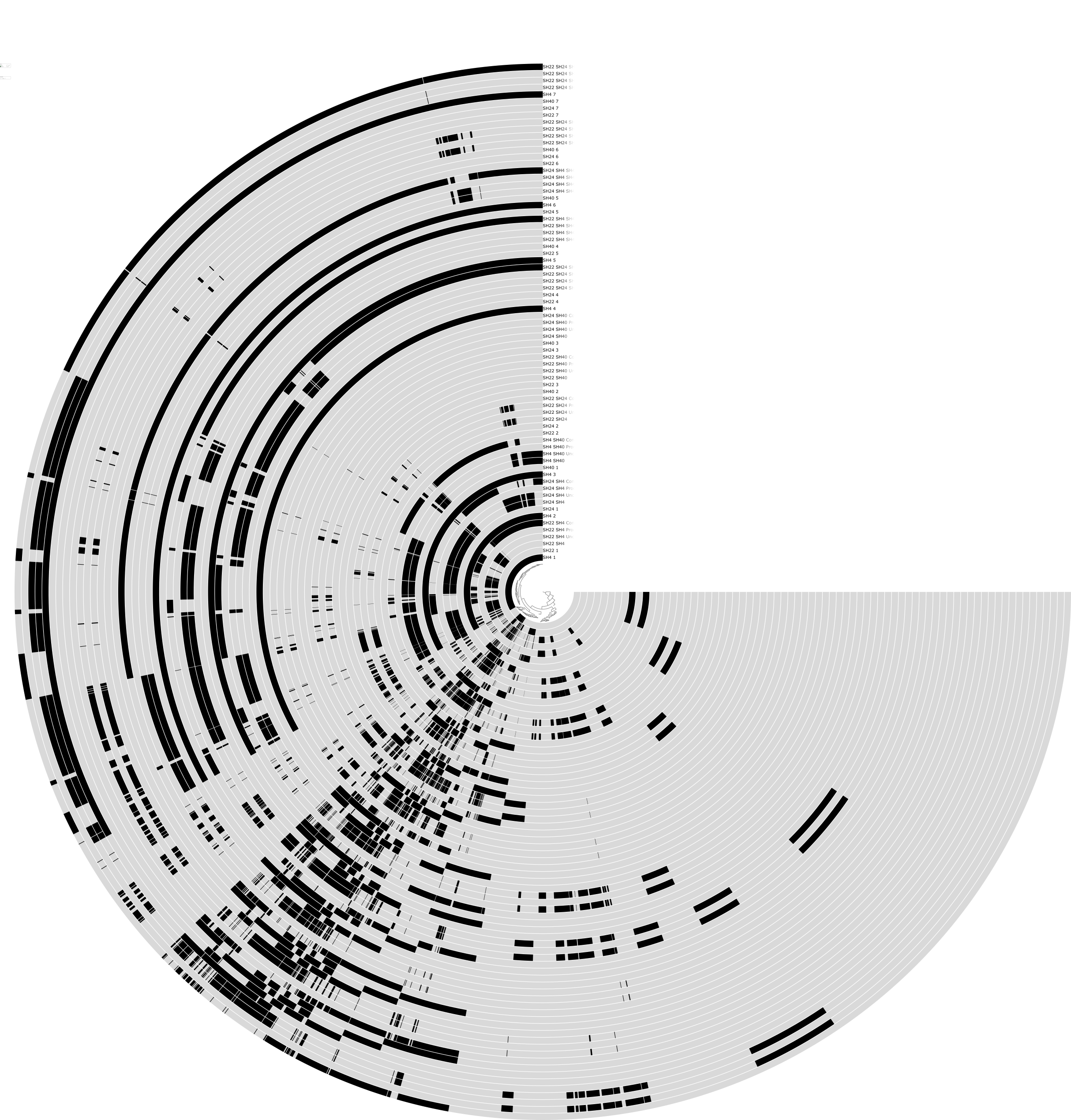
That looks a bit messy, but we will tame it step by step, and add additional data layers to enrich it with useful information.
First of all, you can change the display from “Circle Phylogram” to “Phylogram” to make it more digestible. You can find that option in the settings panel:

Don’t forget to click the ‘Draw’ button again after every change.
Then, find the ‘Options’ tab in the settings panel:

and increase the width of the dendrogram (which will scale the x-axis of the figure) to an appropriate value. I used 8000, but you will likely need to adjust this based on your dataset.
When you hit Draw again, you will see this display:
Slightly better.
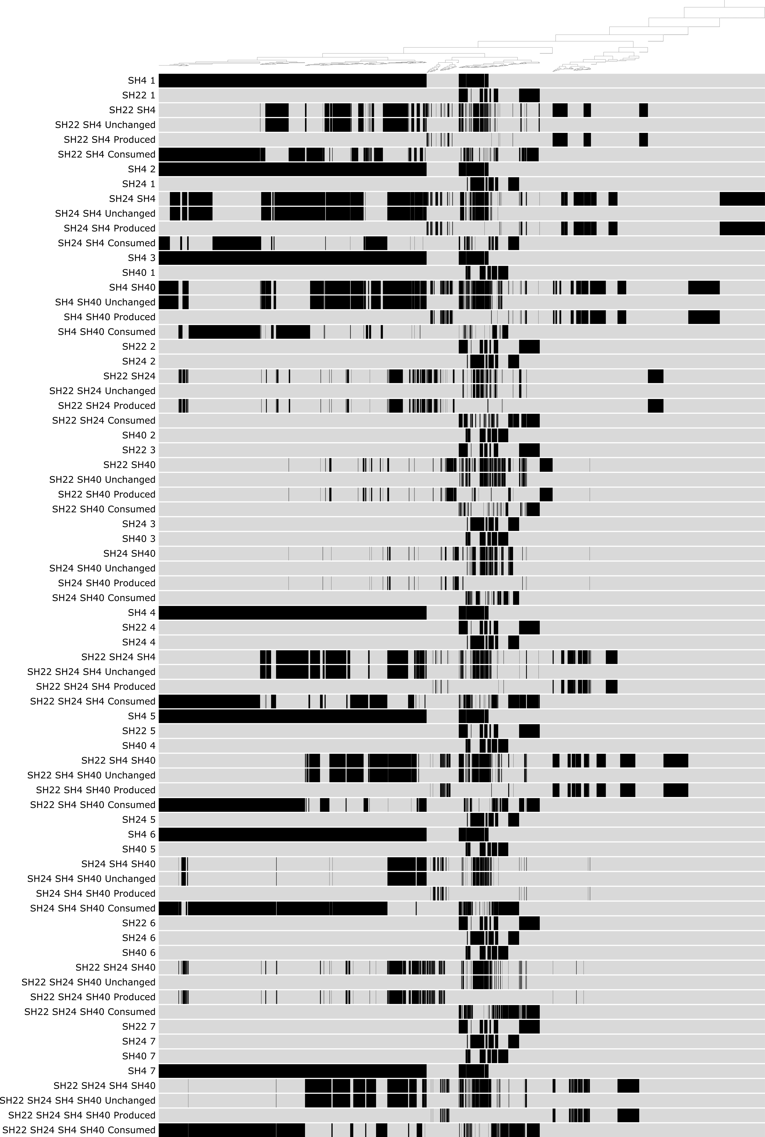
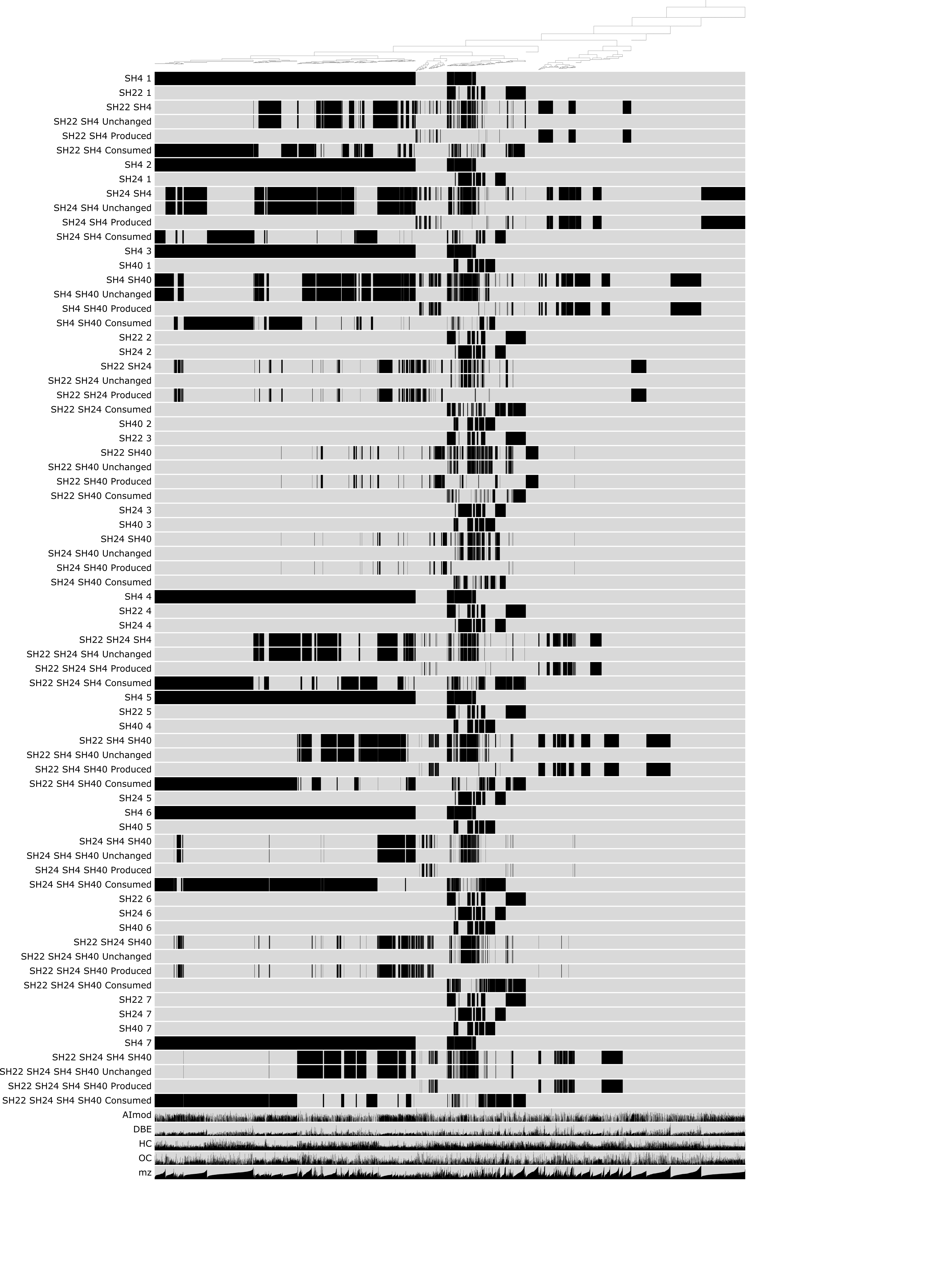
The names of each sample (as we described in the input data file) appear on the left side of each row, and the dendrogram that captures clusters of molecular formulas across these samples (which we generated using the program anvi-matrix-to-newick) appears on top. Each molecular formula is represented by a vertical line within each sample. Because there are so many, they sometimes look like a solid block rather than individual formulas.
As you can already see, the pure culture samples appear several times—this is because we wanted to make it easier to compare the fate of each of those formulas within the microbial consortia. For that purpose, we added consecutive numbers to the sample IDs (i.e., SH4_1, SH4_2, etc.); otherwise, anvi’o would have complained that the input data file contained the same column name multiple times.
This is just the first visualization of the data, but there is more work to be done to make it actually useful and visually appealing—starting with adding additional data layers to enrich the display.
Adding additional data layers for ‘items’ (molecular formula)
This visualization of our data shows that the fate of a molecular formula produced by a given bacterial culture was variable across the different consortia. This differential distribution of molecular formulas across all consortia indicates different kinds and varying degrees of microbial interactions. The figure already conveys a lot of information, but it would be helpful to add additional data layers. In this case, we wanted to show a selection of attributes for each molecular formula (or item). The item-specific data included the mass, the H/C and O/C ratios, double bond equivalents (DBE), and the modified aromaticity index. These data need to be displayed for each molecular formula and therefore must be added as an additional data layer below (or above).
First of all, we need to go back to our terminal, where we can store further information in our profile.db. To make sure that the next time I open anvi-interactive, the display looks the same and doesn’t revert to the default circular phylogram, we need to save the current state of the display. To do this, under the main menu, choose the “Save” option under “State”. anvi-interactive will open a pop-up window like the one below, where we can store the current settings under the “default” state, which will be automatically loaded the next time we run anvi-interactive. Alternatively, you can give the state a different name and use the “Load” option later when needed.

For now, I will close the anvi-interactive tab and return to my terminal, where I press CTRL+C to terminate the runnig server (so we can get our command prompt back).
To add further for our items information, we use the program anvi-import-misc-data, which allows us to add all kinds of additional data to a given profile.db. In this case, we will use the parameter --target-table with the value items to tell anvi’o that these data are associated with each item, representing each molecular formula in our dataset. This is an example input data file for the items additional data:
| formula | mz | HC | OC | AImod | DBE |
|---|---|---|---|---|---|
| C5H4O2 | 95.01385551 | 0.8 | 0.4 | 0.75 | 4 |
| C6H8O | 95.05024127 | 1.333 | 0.167 | 0.45 | 3 |
| C5H6O2 | 97.02949596 | 1.2 | 0.4 | 0.5 | 3 |
| C4H7NO2 | 100.0404053 | 1.75 | 0.5 | 0 | 2 |
| C4H6O3 | 101.0244172 | 1.5 | 0.75 | 0.2 | 2 |
| C8H6 | 101.0396689 | 0.75 | 0 | 0.75 | 6 |
| C4H9NO2 | 102.0560543 | 2.25 | 0.5 | 0 | 1 |
| (…) | (…) | (…) | (…) | (…) | (…) |
Essentially it should be a TAB-delmited file where the left-most column should match exactly with the item identifiers in our “molecular formula distribution spreadsheet”, so that anvi’o can associate the information across both tables.
If you are following this tutorial with the example datasets I provided at the beginning, you already have the items-additional-data.txt file in your work directory, and you can import it into the profile.db using the program anvi-import-misc-data with this command:
anvi-import-misc-data items-additional-data.txt \
                      -p profile.db \
                      --target-table items
And use the same command as before to start anvi-interactive, this time including the new data:
anvi-interactive -d data.txt \
                 -t dendrogram.newick \
                 -p profile.db \
                 --manual
And this is what our figure looks like now:
At the bottom, we now have five additional layers of information for each molecular formula. At least in this specific case, no clear pattern becomes apparent. This is probably because we clustered the molecular formulas based on their distribution across samples and not their specific fate (production, consumption, preservation), which might reveal clearer patterns. Maybe we can use this information in another analysis :)
For now, we decided to remove these layers from the display again. To do that, we can simply set the height of each layer to 0 under the “DISPLAY” menu, which is the easy way :)
You can also remove any data layer you no longer wish to see in the interface using the program anvi-delete-misc-data. But I chose the lazy option, and after hitting “DRAW”, I was left with the same display I started with.
While additional item data wasn’t useful for this particular analysis, other analyses may benefit from this kind of additional information, so I decided to explain how to add it nevertheless.
Adding additional data layers for ‘layers’ (samples)
We haven’t run out of interesting data to show yet, though. However, the kind of data we want to include in the display now is not specifically associated with each molecular formula, but with each sample. For example: the observed molecular formula count, the predicted molecular formula count, the relative fraction of consumed, produced, and unchanged molecular formulas, and the relative abundances of the different bacterial isolates within each of the consortia.
To do this, we first need to generate a spreadsheet where the first column contains the sample identifier. The sample identifier must be identical to the sample identifier in our original dataset so that anvi’o can correctly match the information. The following columns can contain any data we wish to add, with each column’s first row containing a data identifier. For example, our first data column contains MF_Count_Total, which represents the overall molecular formula count in each sample.
Again, if you are following this tutorial with the example datasets I provided at the beginning, you already have the layers-additional-data.txt file in your work directory, and it looks like this:
| samples | MF_Count_Total | Total_Predicted_compounds | stacked_bar_3!Relative_Gained | stacked_bar_3!Relative_Lost | stacked_bar_3!Relative_Unchanged | Strain_No | stacked_bar_2!SH4 | stacked_bar_2!SH22 | stacked_bar_2!SH24 | stacked_bar_2!SH40 | stacked_bar_2!NA |
|---|---|---|---|---|---|---|---|---|---|---|---|
| SH22_SH4 | 1172 | 2418 | 0 | 0 | 0 | 2 | 94.74188769 | 4.897643694 | 0 | 0 | 0 |
| SH22_SH4_Consumed | 1528 | 0.104444444 | 0.565925926 | 0.32962963 | 2 | 94.74188769 | 4.897643694 | 0 | 0 | 0 | |
| SH22_SH4_Produced | 282 | 0.104444444 | 0.565925926 | 0.32962963 | 2 | 94.74188769 | 4.897643694 | 0 | 0 | 0 | |
| SH22_SH4_Unchanged | 890 | 0.104444444 | 0.565925926 | 0.32962963 | 2 | 94.74188769 | 4.897643694 | 0 | 0 | 0 | |
| SH24_SH4 | 2228 | 2359 | 0 | 0 | 0 | 2 | 84.98297828 | 0 | 15.01702172 | 0 | 0 |
| SH24_SH4_Consumed | 853 | 0.2343395 | 0.276858163 | 0.488802337 | 2 | 84.98297828 | 0 | 15.01702172 | 0 | 0 | |
| SH24_SH4_Produced | 722 | 0.2343395 | 0.276858163 | 0.488802337 | 2 | 84.98297828 | 0 | 15.01702172 | 0 | 0 | |
| SH24_SH4_Unchanged | 1506 | 0.2343395 | 0.276858163 | 0.488802337 | 2 | 84.98297828 | 0 | 15.01702172 | 0 | 0 | |
| SH4_SH40 | 2021 | 2353 | 0 | 0 | 0 | 2 | 92.23433637 | 0 | 0.651445616 | 7.114218013 | 0 |
| SH4_SH40_Consumed | 1026 | 0.227765015 | 0.336724647 | 0.435510338 | 2 | 92.23433637 | 0 | 0.651445616 | 7.114218013 | 0 | |
| SH4_SH40_Produced | 694 | 0.227765015 | 0.336724647 | 0.435510338 | 2 | 92.23433637 | 0 | 0.651445616 | 7.114218013 | 0 | |
| SH4_SH40_Unchanged | 1327 | 0.227765015 | 0.336724647 | 0.435510338 | 2 | 92.23433637 | 0 | 0.651445616 | 7.114218013 | 0 | |
| SH22_SH24 | 666 | 502 | 0 | 0 | 0 | 2 | 0 | 26.73233467 | 71.66178347 | 0.423239989 | 1.773962804 |
| SH22_SH24_Consumed | 355 | 0.508325171 | 0.347698335 | 0.143976494 | 2 | 0 | 26.73233467 | 71.66178347 | 0.423239989 | 1.773962804 | |
| SH22_SH24_Produced | 519 | 0.508325171 | 0.347698335 | 0.143976494 | 2 | 0 | 26.73233467 | 71.66178347 | 0.423239989 | 1.773962804 | |
| SH22_SH24_Unchanged | 147 | 0.508325171 | 0.347698335 | 0.143976494 | 2 | 0 | 26.73233467 | 71.66178347 | 0.423239989 | 1.773962804 | |
| SH22_SH40 | 554 | 451 | 0 | 0 | 0 | 2 | 0 | 63.3282025 | 11.75311559 | 24.80543162 | 0 |
| SH22_SH40_Consumed | 204 | 0.405013193 | 0.269129288 | 0.32585752 | 2 | 0 | 63.3282025 | 11.75311559 | 24.80543162 | 0 | |
| SH22_SH40_Produced | 307 | 0.405013193 | 0.269129288 | 0.32585752 | 2 | 0 | 63.3282025 | 11.75311559 | 24.80543162 | 0 | |
| SH22_SH40_Unchanged | 247 | 0.405013193 | 0.269129288 | 0.32585752 | 2 | 0 | 63.3282025 | 11.75311559 | 24.80543162 | 0 | |
| SH24_SH40 | 296 | 399 | 0 | 0 | 0 | 2 | 0 | 32.57275966 | 40.47564686 | 26.40763396 | 0 |
| SH24_SH40_Consumed | 203 | 0.200400802 | 0.406813627 | 0.392785571 | 2 | 0 | 32.57275966 | 40.47564686 | 26.40763396 | 0 | |
| SH24_SH40_Produced | 100 | 0.200400802 | 0.406813627 | 0.392785571 | 2 | 0 | 32.57275966 | 40.47564686 | 26.40763396 | 0 | |
| SH24_SH40_Unchanged | 196 | 0.200400802 | 0.406813627 | 0.392785571 | 2 | 0 | 32.57275966 | 40.47564686 | 26.40763396 | 0 | |
| SH22_SH24_SH4 | 1278 | 2527 | 0 | 0 | 0 | 3 | 82.77036875 | 5.731805077 | 10.08200592 | 0 | 3.924284395 |
| SH22_SH24_SH4_Consumed | 1530 | 0.100071225 | 0.544871795 | 0.35505698 | 3 | 82.77036875 | 5.731805077 | 10.08200592 | 0 | 3.924284395 | |
| SH22_SH24_SH4_Produced | 281 | 0.100071225 | 0.544871795 | 0.35505698 | 3 | 82.77036875 | 5.731805077 | 10.08200592 | 0 | 3.924284395 | |
| SH22_SH24_SH4_Unchanged | 997 | 0.100071225 | 0.544871795 | 0.35505698 | 3 | 82.77036875 | 5.731805077 | 10.08200592 | 0 | 3.924284395 | |
| SH22_SH4_SH40 | 1570 | 2515 | 0 | 0 | 0 | 3 | 90.77609826 | 3.247378359 | 0 | 5.976523381 | 0 |
| SH22_SH4_SH40_Consumed | 1567 | 0.19827861 | 0.499521836 | 0.302199554 | 3 | 90.77609826 | 3.247378359 | 0 | 5.976523381 | 0 | |
| SH22_SH4_SH40_Produced | 622 | 0.19827861 | 0.499521836 | 0.302199554 | 3 | 90.77609826 | 3.247378359 | 0 | 5.976523381 | 0 | |
| SH22_SH4_SH40_Unchanged | 948 | 0.19827861 | 0.499521836 | 0.302199554 | 3 | 90.77609826 | 3.247378359 | 0 | 5.976523381 | 0 | |
| SH24_SH4_SH40 | 534 | 2448 | 0 | 0 | 0 | 3 | 91.50290424 | 0 | 4.176210397 | 4.320885364 | 0 |
| SH24_SH4_SH40_Consumed | 1981 | 0.026640159 | 0.787673956 | 0.185685885 | 3 | 91.50290424 | 0 | 4.176210397 | 4.320885364 | 0 | |
| SH24_SH4_SH40_Produced | 67 | 0.026640159 | 0.787673956 | 0.185685885 | 3 | 91.50290424 | 0 | 4.176210397 | 4.320885364 | 0 | |
| SH24_SH4_SH40_Unchanged | 467 | 0.026640159 | 0.787673956 | 0.185685885 | 3 | 91.50290424 | 0 | 4.176210397 | 4.320885364 | 0 | |
| SH22_SH24_SH40 | 629 | 604 | 0 | 0 | 0 | 3 | 0 | 30.47393048 | 62.68516164 | 6.840907884 | 0 |
| SH22_SH24_SH40_Consumed | 413 | 0.420345489 | 0.396353167 | 0.183301344 | 3 | 0 | 30.47393048 | 62.68516164 | 6.840907884 | 0 | |
| SH22_SH24_SH40_Produced | 438 | 0.420345489 | 0.396353167 | 0.183301344 | 3 | 0 | 30.47393048 | 62.68516164 | 6.840907884 | 0 | |
| SH22_SH24_SH40_Unchanged | 191 | 0.420345489 | 0.396353167 | 0.183301344 | 3 | 0 | 30.47393048 | 62.68516164 | 6.840907884 | 0 | |
| SH22_SH24_SH4_SH40 | 1321 | 2602 | 0 | 0 | 0 | 4 | 87.31686287 | 3.213122083 | 2.994942931 | 4.576866026 | 5.694618273 |
| SH22_SH24_SH4_SH40_Consumed | 1649 | 0.125042474 | 0.560312606 | 0.31464492 | 4 | 87.31686287 | 3.213122083 | 2.994942931 | 4.576866026 | 5.694618273 | |
| SH22_SH24_SH4_SH40_Produced | 368 | 0.125042474 | 0.560312606 | 0.31464492 | 4 | 87.31686287 | 3.213122083 | 2.994942931 | 4.576866026 | 5.694618273 | |
| SH22_SH24_SH4_SH40_Unchanged | 926 | 0.125042474 | 0.560312606 | 0.31464492 | 4 | 87.31686287 | 3.213122083 | 2.994942931 | 4.576866026 | 5.694618273 |
To add data as stacked bars (such as relative abundances based on 16S rRNA gene amplicon data) we need to let anvi’o know our intention by naming the corresponding columns and values in a particular way. You can find more information about the formatting here. But I will seimply use a prefix, stacked_bar, followed by a mandatory ! character, followed by a specific sample identifier. For example, in this case, the first column that contains stacked bar data is called stacked_bar_2!SH22, and the next column would be stacked_bar_2!SH24. This way, anvi’o knows that these columns belong together.
We again use anvi-import-misc-data, but this time we use the flag --target-table layers to indicate that this information is sample-specific and should be matched to each sample.
Before we proceed, we need to save the current state and terminate the server using CTRL+C. Then, we can add the data using the following command:
anvi-import-misc-data layers-additional-data.txt \
                      -p profile.db \
                      --target-table layers
And run anvi-interactive again to see its effect:
anvi-interactive -d data.txt \
                 -t dendrogram.newick \
                 -p profile.db \
                 --manual
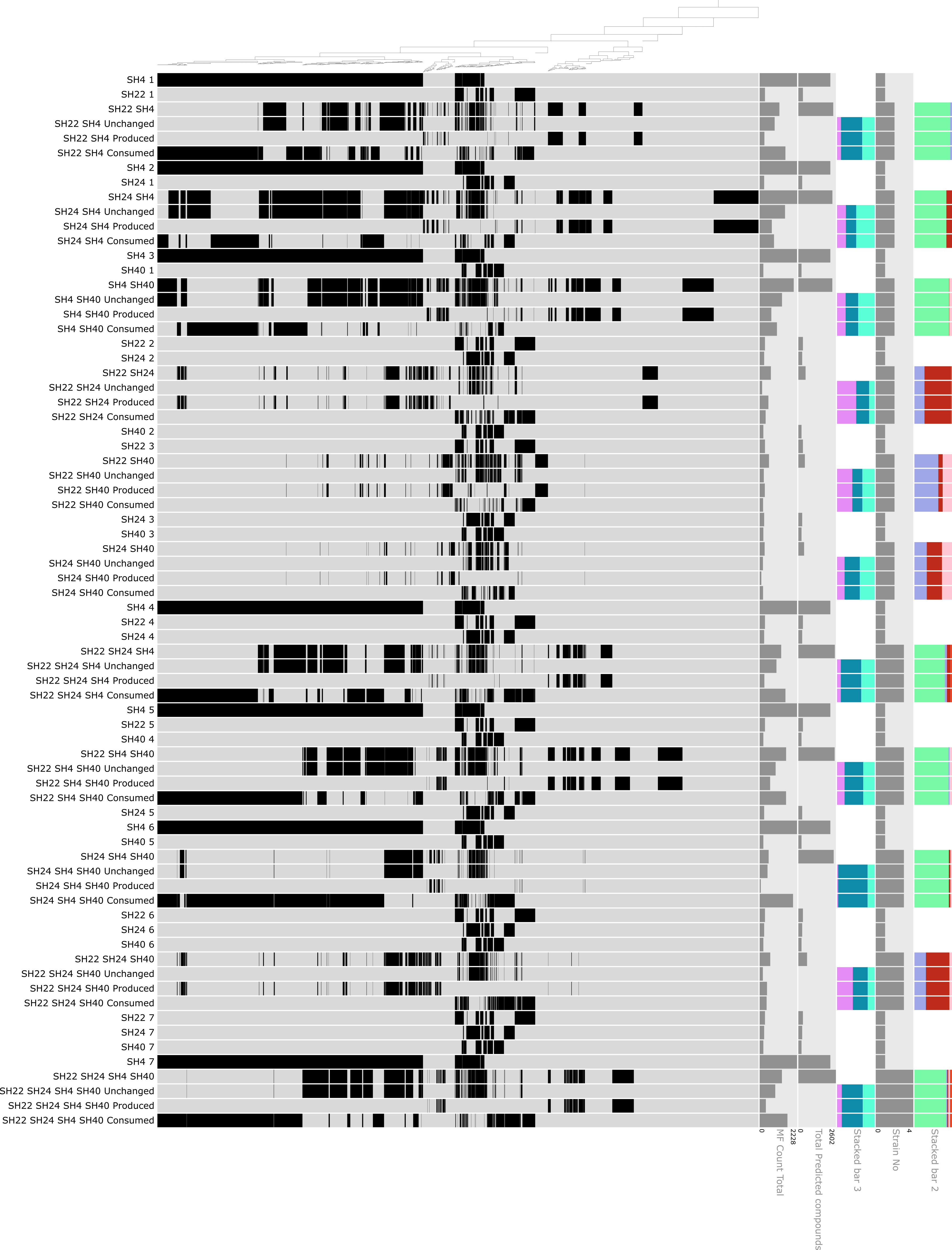
Now, the additional data are visible and aligned with each sample on the right side of the figure! :)
Fine-tuning the display aesthetics for better structure and clarity
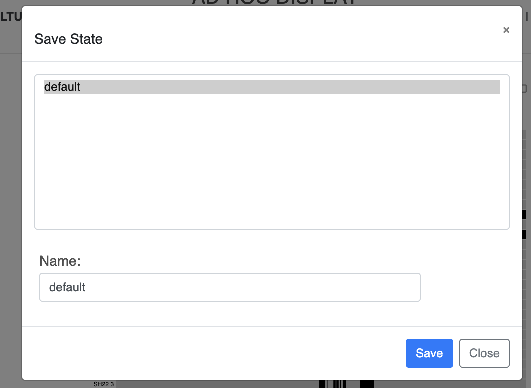
Aside from the annotations—which we will later change outside of anvi-interactive—we can use colors to structure the visualization more clearly. We have 11 different microbial consortia. To discern which data belong to which microbial consortium, I generated a color palette using this tool (which only allows a 10-color palette, so I added another hue manually):
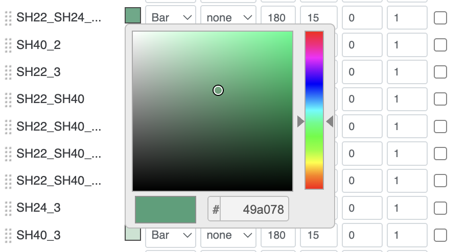
In the main menu of anvi-interactive, under “DISPLAY,” we can manually change the color used for each sample by clicking on the (currently black) square next to “color” and pasting the HEX code for each color into the small window in the lower right:
At some point my display lookedlike this, pretty colorful, and containing all the information:
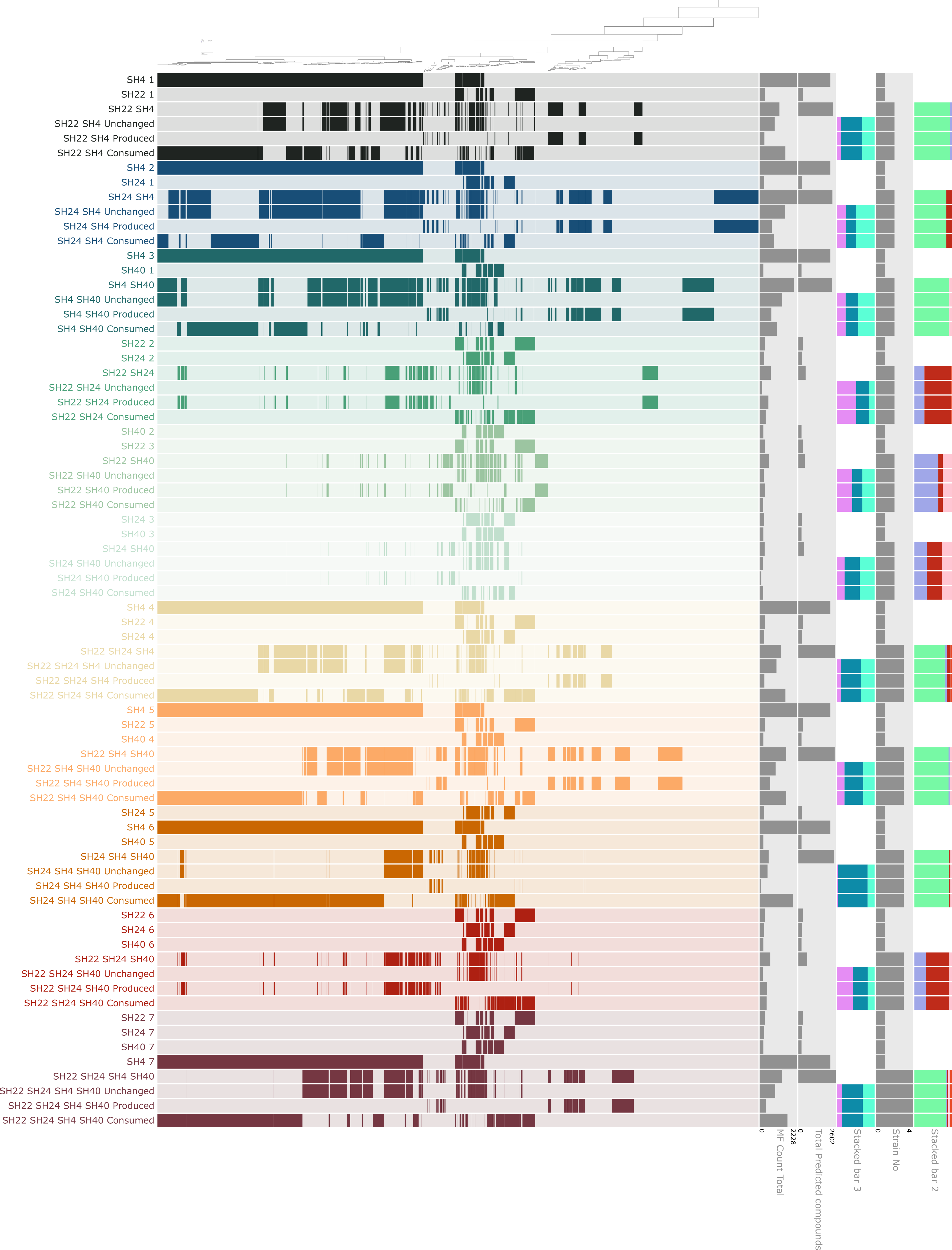
Then it evolved further with the removal of some layers that didn’t seem to contribute much to the story we wished to tell, changing colors to make it easier for people to follow in a paper format, etc.
Then I exported the display that I was comfortable with, and brought it to Inkscape to continue working with it. Inkscape is an open-source and free SVG editor, but you can edit anvi’o interactive interface exports in any vector graphics editor.
The final figure looks like this:
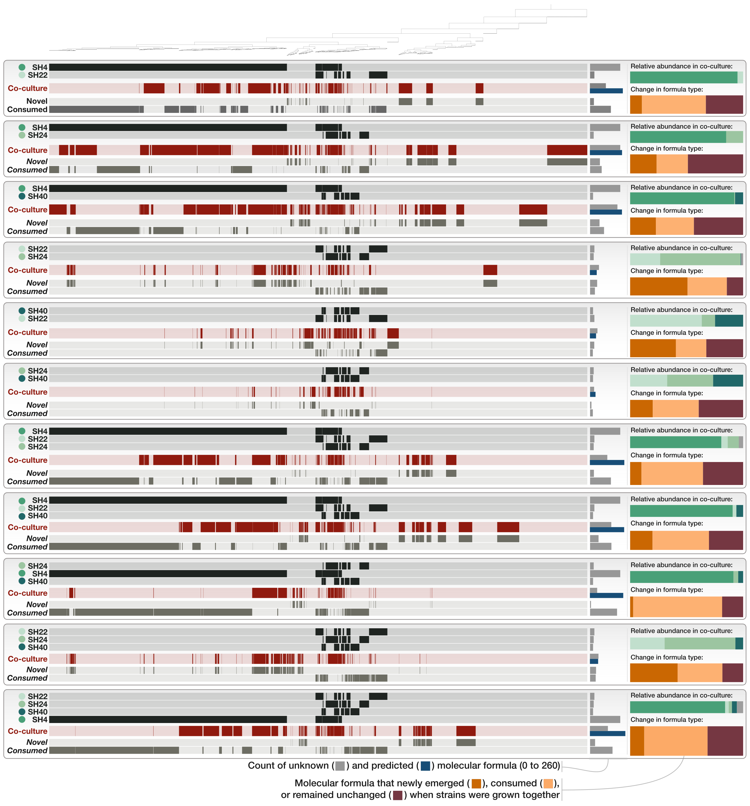
The figure shows the distribution of molecular formulas that are clustered based on their occurrence across pure cultures and microbial consortia. For each co-culture, rows in black show the molecular formulas produced by the respective bacterial isolate, rows in red show the molecular formulas observed in the respective co-culture and rows in light grey highlight novel and consumed molecular formulas. The dark grey bars on the right side show the molecular formula count for each culture and co-culture along with the predicted molecular formula count in dark blue and the number of preserved, produced and consumed molecular formulas in dark grey. The green stacked bars show the relative abundance of each isolate in the co-cultures, with SH4 in green, SH22 in light blue-green, SH24 in turquoise and SH40 in dark green. The orange stacked bars below show the relative contribution of novel (orange), consumed (peach) and preserved (dark red) molecular formulas in the respective co-cultures.
Conclusion
For our project, we learned a lot from this visualization that helped us interpret the data. Additionally, this figure contains information that we would have usually split across several individual figures, but bringing everything together in one display made it much easier to describe and discuss the observations.
I hope this tutorial gives you some inspiration as well as practical means to visualize your own mass-spec data in anvi’o. If anything was unclear, please feel free to comment below, reach out to me directly, or write to the anvi’o community on Discord. Thanks for reading!