anvi-draw-kegg-pathways

Write KEGG pathway map files incorporating data sourced from external inputs.

🔙 To the main page of anvi’o programs and artifacts.

Authors

Requires

kegg-data

Can use

contigs-db external-genomes pan-db genomes-storage-db reaction-network-json kegg-reaction-txt kegg-compound-txt kegg-membership-colors-txt kegg-value-colors-txt

Provides

kegg-pathway-map kegg-slice-key-txt

Usage

anvi-draw-kegg-pathways draws kegg-pathway-map files from input kegg-reaction-txt and/or kegg-compound-txt files, one or more contigs-dbs, a pan-db, or a metabolic model file (see reaction-network-json). The visualization of user data in the context of KEGG’s curated biochemical pathways can reveal patterns in metabolism.

Setup

There are hundreds of pathway maps, listed and categorized here. anvi-setup-kegg-data downloads, among other files, the maps with corresponding XML files that allow elements of the map to be modified. The following command sets up the database in a default anvi’o directory.

Additional Python packages may be needed if you installed anvi’o before this program’s package requirements were included. These can be installed with the following command.

The program can be tested with the following command.

Download newest available files

Alternatively, KEGG data can be set up not from a snapshot but by downloading the newest files available from KEGG using the -D flag. In the following command, a higher number of download threads than the default of 1 is provided by -T, which significantly speeds up downloading.

Install in non-default location

To preserve KEGG data that you’ve already set up for whatever reason, the new snapshot or download can be placed in a non-default location using the option, --kegg-data-dir.

anvi-draw-kegg-pathways requires a --kegg-dir argument to seek KEGG data in a non-default location.

Pathway selection

By default, this program draws the maps that contain data of interest, e.g., KO gene sequence annotations in a contigs-db.

To draw all maps available in kegg-data, including those that don’t contain data of interest, use the flag, --draw-bare-maps.

The option, --pathway-numbers, limits the output to maps of interest. A single ID number can be provided, e.g., 00010 for Glycolysis / Gluconeogenesis, or multiple numbers can be listed, e.g., 00010 00020. Regular expressions can also be provided, e.g., 011.. 01[23].., where . represents any character: here the set of numbers given by 011.. corresponds to “global” maps and 01[23].. to “overview” maps.

The following command would draw all global maps and the glycolysis map, regardless of whether they contain any anvi’o data of interest (here, KO annotations from a contigs database).

Labels

By default, the reaction elements of standard maps are labeled, and nothing else is. Most of these are boxes. A few standard maps, such as N-Glycan biosynthesis (00510), also draw reactions as lines, which are labeled too. The fill of a box hides the text of the base map, so a box without a label is blank. --reaction-labels and --compound-labels choose the kinds of map whose reaction elements and compound circles are labeled. Each takes one or more of standard, overview, and global, or none for no labels. Global maps are numbered 011XX, overview maps are numbered 012XX and 013XX, and all other maps are standard (see Single contigs database for an example of each).

The kinds given replace the default. The following command labels the reaction elements of standard maps, the reaction arrows of overview maps, and the compound circles of both kinds of map.

Every element of a map of a given kind is labeled, with or without data. A reaction element is labeled with KEGG’s name for it. That is the first KO of the element, followed by ... when the element stands for several KOs. The label may therefore name a KO that is not in your data. It is a KO even when a kegg-reaction-txt file holds KEGG reaction IDs. A compound circle is labeled with the KEGG ID of its compound, glycan, or drug, or with the first of several IDs, followed by ....

A compound label is wider than its circle and sits above its center. It can cover nearby lines, arrowheads, boxes, and the compound names printed on the base map. A compound that takes part in no reaction on the map is labeled in faint gray. On maps without reactions, such as many signaling maps, that is every compound. The labels of global maps are small and crowded, and they can be read only when the map is zoomed in.

Output

This program requires the path to a directory as an argument to -o or --output-dir. This must be a non-existent directory unless the flag, -W or --overwrite-output-destinations, is also used. Options are available to make it easier to browse through output files and anticipate their contents.

Directory layout

Map files are sorted into up to four subdirectories, one for each kind of map:

Subdirectory	Contents
unified	The type of map drawn from all of the data at once. With a single source — a kegg-reaction-txt and/or kegg-compound-txt with no sample column, one contigs-db, or one reaction-network-json — these maps per pathway are the only ones drawn. Not written at all with --skip-unified-maps.
individual	One subdirectory per data source, named after it: each sample of a text file, each contigs database, each genome of a pangenome, or, when they are grouped with a groups-txt file, each group instead. Drawn on request with --draw-individual-files.
grid	The map grids, each showing the unified map alongside the individual ones, or the individual ones alone with --skip-unified-maps. Drawn on request with --draw-grid.
by_map	The same individual maps arranged the other way round: one subdirectory per map, each holding one file per data source, named after it. Written on request with --collate-files-by-map. With --animate-files-by-map, a player of each map is written beside its subdirectory.

Colorbars, which are keys to the colors of every map in the run, are written at the top of the output directory beside these subdirectories. The reaction layer can have the keys below. The compound layer has the same colorbars, with compounds in place of reactions.

File	What it keys
colorbar_reactions.pdf	The fills of the unified map. For a file without a sample column, it keys the fills of every map.
colorbar_reactions_samples.pdf or colorbar_reactions_groups.pdf	The fills of the maps of the individual samples or groups, which share this key.
colorbar_reactions_border.pdf	The borders of the unified map, or of every map for a file without a sample column (see Color borders by a second column).
colorbar_reactions_border_samples.pdf or colorbar_reactions_border_groups.pdf	The borders of the maps of the individual samples or groups, which share this key.
slice_key_reactions.txt	A kegg-slice-key-txt that lists each slice drawn with --reaction-slice-by (see Draw elements in slices).
slice_key_reactions_border.txt	A kegg-slice-key-txt that lists each slice of the rings drawn with --reaction-border-slice-by (see Slice rings).

A group’s own maps that count the group’s sources are keyed beside them instead, in individual and grid (see Show individual group maps).

Because the names in individual come from your own data, they are kept in that subdirectory of their own: a sample, genome, or group may be named anything at all — including unified, grid, by_map, all_maps, or Metabolism — without ever colliding with a directory this program creates for itself.

The one requirement is that a name becoming a subdirectory has to work as a directory name, so a name containing a path separator, such as Rhizobium meliloti RU11/001, is refused. This only applies to the sources that are actually drawn individually: a source summarized on the unified map contributes color rather than a path, so its name is never used as one, and a source left out of a subset requested with --draw-individual-files or --draw-grid is not checked either.

File names

By default, an output file is named after the map’s KEGG accession, e.g., ko00010.pdf for Glycolysis / Gluconeogenesis. The --name-files flag attaches a simplified version of the pathway name to the file name, e.g., ko00010_Glycolysis_Gluconeogenesis.pdf.

File categorization

The --categorize-files flag categorizes output map files into a subdirectory structure based on the KEGG BRITE hierarchy of pathways. For example, a Glycolysis / Gluconeogenesis map would be placed in a directory named Metabolism/Carbohydrate_metabolism, as would a Citrate cycle (TCA cycle) map, whereas an RNA polymerase map would be placed in a directory named Genetic_Information_Processing/Transcription. These category directories are built inside each of the subdirectories described above, so a categorized map of one sample would be found at, say, individual/SAMPLE_1/Metabolism/Carbohydrate_metabolism/ko00010.pdf. Within unified, individual, and grid, a subdirectory named all_maps is created alongside them, holding a hard link to every one of that directory’s maps so that they can also be reached from a single place.

Skipping the summary map

The unified map summarizes every sample, group, contigs database, or genome at once. A run draws it even when no summary was asked for. By default the sources are summarized by presence. That summary is not always wanted, and it can claim more than the data supports. Pooling values is only meaningful across commensurable samples. Presence in any one sample says little when the point is to compare the samples.

--skip-unified-maps leaves that map out. The unified subdirectory is not written. The colorbar for that map is not written either, unless the same scale also colors the individual maps, which would otherwise have no key anywhere in the output. The same rule applies to the key of the borders of that map, such as colorbar_reactions_border.pdf. The maps of the individual sources are all that is left, so --draw-individual-files and/or --draw-grid are required. Each grid holds the individual maps alone, without the first ‘unified’ map panel labeled all (or pangenome).

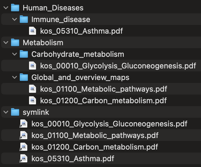
Here is a simple example of the output file structure produced with --name-files and --categorize-files in the course of anvi-self-test --suite kegg-mapping (with the -o option to save the temporary directories in the test from removal).

Gathering files by map

--draw-individual-files writes one subdirectory per data source, each holding that source’s whole set of maps. That is the right arrangement for reading everything about one sample, and the wrong one for comparing a single map across samples, which means opening one file in each of those subdirectories. The --collate-files-by-map flag adds the transposed view: a subdirectory named after each map, holding one file per source, named after the source.

With samples A through E, by_map/ko00010 holds A.pdf through E.pdf, by_map/ko00020 holds another five files, and so on. Selecting everything in one of those subdirectories and stepping through it with a file browser’s preview shows the colors of a single map changing from sample to sample, like an animation. Files are sorted by the name of their source, so name your samples in the order in which you would like to step through them.

This is a second arrangement of the same files rather than a replacement: the subdirectory per source stays where it is, and the gathered files are links to the maps already drawn there, so they take up no disk space of their own. --name-files and --categorize-files apply here as they do elsewhere in the output, so with both of them a gathered map would be found at, say, by_map/Metabolism/Carbohydrate_metabolism/ko00010_Glycolysis_Gluconeogenesis/SAMPLE_1.pdf.

Playing maps gathered by map

The --animate-files-by-map flag adds a player for each map gathered by --collate-files-by-map. The player is an HTML file written beside the map’s subdirectory, so by_map/ko00010 gets by_map/ko00010.html. It opens in any current web browser, straight from the disk, with no internet connection and no anvi’o installation, so it can be passed around as a single file.

The player shows the map of each sample, contigs database, genome, or group in turn. The Play button or the space bar starts and pauses it. Dragging the slider moves back and forth to any frame, the arrow keys step one frame at a time, and Home and End jump to the first and last frames. The seconds per frame and looping can be changed on the page. Actual size shows the map at its full resolution instead of fitting it to the window.

The name of each frame’s source is shown above the map. Frames follow the order of the run. Samples are sorted by name as text, so T10 comes before T2 unless the numbers are padded, as in T02. Groups follow the groups-txt file, contigs databases follow the order in which they were given, and genomes follow the pangenome. Names listed after --draw-individual-files are shown in the order listed, which is a way to choose any order.

A source with no data on a map has no file in that map’s subdirectory. The player shows the bare map in its place, with the note “No data on this map”, so every player of a run has the same frames in the same order. With --draw-bare-maps, the bare map of that source is drawn and gathered like any other map, so the player shows it without the note. Every map of the run then gets a player, even a map with no data in any source.

The colorbars that key the individual maps are shown beside the map. Where groups are colored by counts of their own sources, each group has its own colorbar, and the player shows the one that belongs to the frame.

Each frame is stored in the page as a lossless image of the map at the resolution of the KEGG image, so the colors are those of the map files. Unlike the gathered maps, the players are new files rather than links. Three frames of 00010 take about 0.2 MB, and twelve frames of the global map 01100 take about 13 MB.

Mapping reaction and compound occurrence

Gene sequences in anvi’o databases can be annotated with KEGG Orthologs (KOs) indicating the functional capabilities of the gene product: see anvi-run-kegg-kofams. KO data can be provided directly by a kegg-reaction-txt file or a reaction network JSON file, instead of through anvi’o databases. KO data from one or more organisms can be mapped, enabling the comparison of metabolic capabilities.

Rather than KOs, KEGG reactions supplied by a kegg-reaction-txt file can be used to draw the reaction layer; both map to reaction elements — reaction lines in global and overview maps and boxes in standard maps.

KEGG compounds provided by a kegg-compound-txt file can be used to draw the compound layer of circle elements on maps.

Reaction and compound text files

Maps can be drawn directly from per-layer text files — the quickest way to visualize custom data, needing no anvi’o database. There is one file per layer, and either or both can be given:

• a kegg-reaction-txt file (--reaction-txt) colors the reaction layer. Its accession column holds either KO IDs (K#####), as with the database inputs, or KEGG reaction IDs (R#####) when data are per-reaction, such as a metabolic model’s fluxes — ALL accessions in the file must be of one type or the other.
• a kegg-compound-txt file (--compound-txt) colors the compound layer, from data such as metabolomics. Its accession column holds compound IDs (C#####).

When both files are given, the two layers are drawn together on each map, each on its own color scale, so that (for example) metabolite levels can be compared against enzyme expression. Each layer is colored independently by its own auto-detected mode (see below). Columns named by --reaction-slice-weights, --reaction-border-column, and --compound-border-column are left out of the detection. Here is a basic command drawing just the reaction layer.

See kegg-reaction-txt and kegg-compound-txt for the full format of each file.

Data from more than one origin, such as multiple genomes or samples, can be compared on the same maps by adding a sample column. Because this works just like comparing multiple contigs databases, it is described further below, under Compare samples in an input text file.

Instead of showing presence/absence, elements can be colored by a continuous quantitative value from a numeric column of the file, such as KO coverage, reaction flux, or compound concentration. This is described below, under Color elements by a quantitative value.

A second column can color the borders of reaction boxes and compound circles. It is named with --reaction-border-column or --compound-border-column, so it is never taken for the value column. This is described below, under Color borders by a second column.

Reaction network JSON file

Pathway maps can be drawn from a reaction network JSON file produced by anvi-reaction-network or anvi-get-metabolic-model-file. This is especially useful with custom enzyme lists — for example, annotations from transcriptomic or proteomic data, or predicted gene content of a last common ancestor.

Single contigs database

Pathway maps can be drawn from KO data in a single contigs-db.

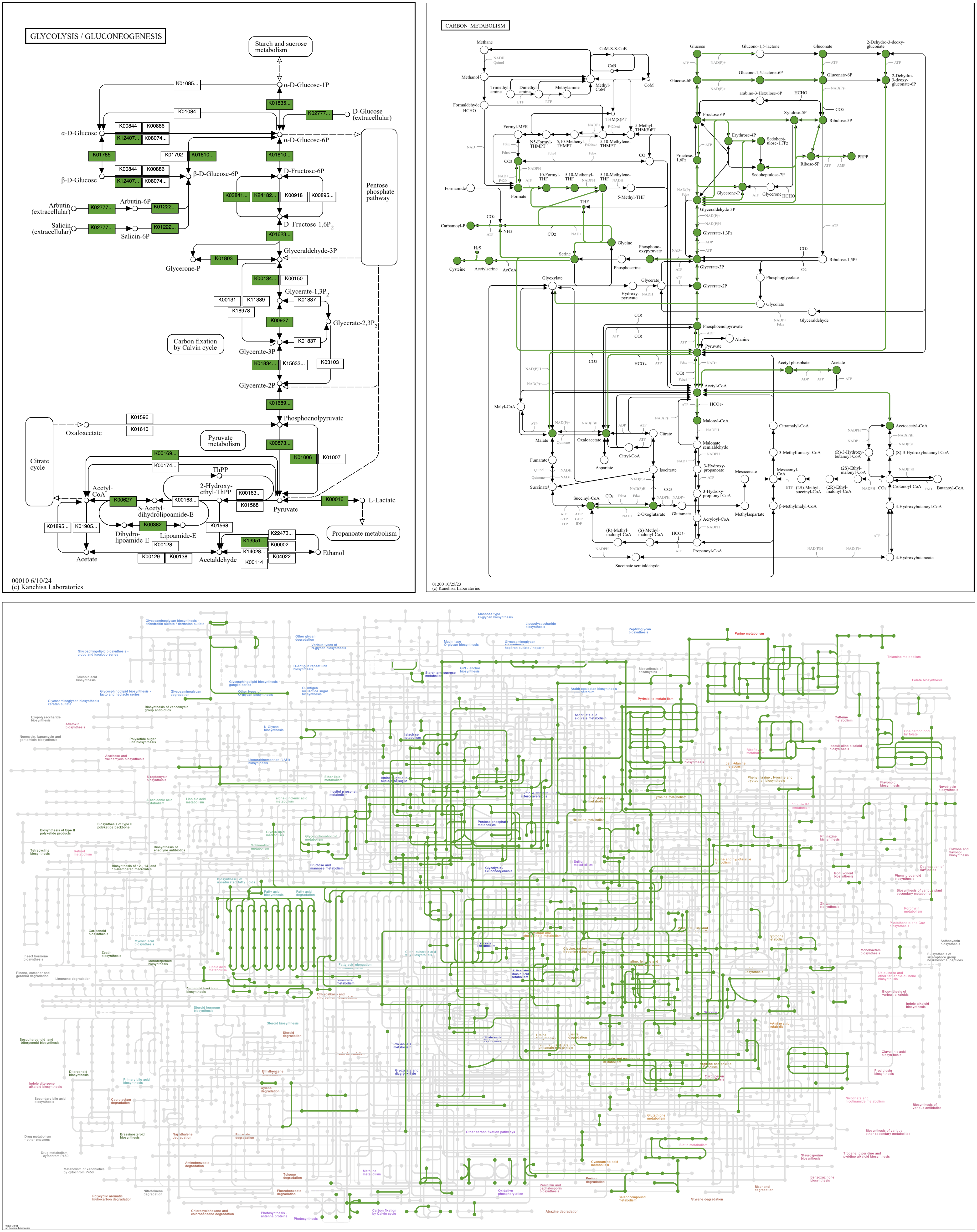
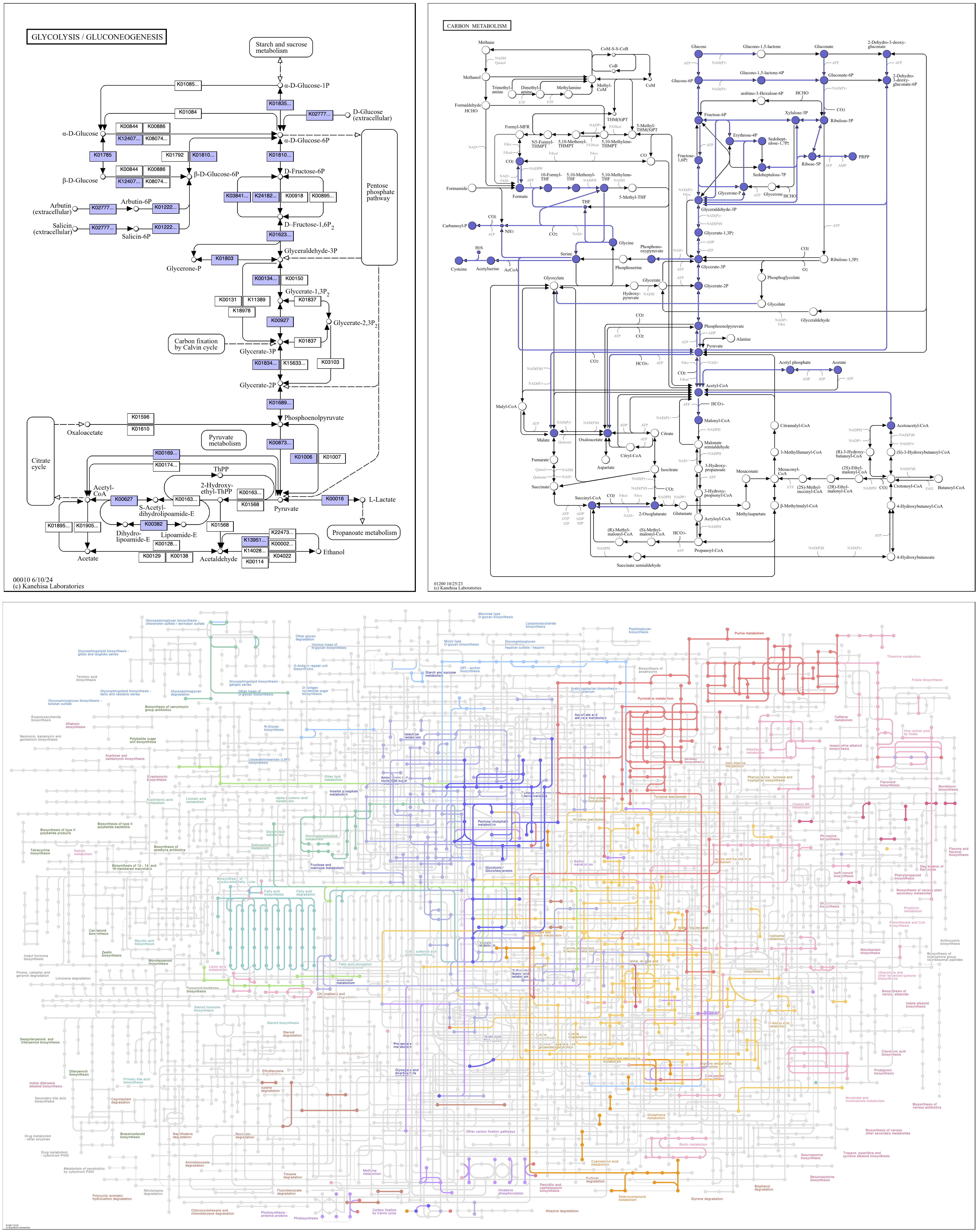
Here are three maps drawn with this command from a bacterial genomic contigs database. The map in the upper left, 00010 Glycolysis / Gluconeogenesis, is a “standard” map, in which boxes are associated with a reaction arrow and one or more KOs. The map in the upper right, 01200 Carbon metabolism, is a metabolic “overview” map. Overview maps have numerical IDs in the range 012XX and 013XX. Reaction arrows in overview maps are associated with one or more KOs and are colored and widened if represented by anvi’o KO data. The bottom map, 01100 Metabolic pathways, is a “global” metabolic map. Global maps have numerical IDs in the range 011XX. Reaction lines in global maps are associated with one or more KOs and colored if represented by anvi’o KO data. In global and overview maps, a circle is colored where a colored reaction touches it. A reaction touches the circles at the ends of its lines: global maps draw lines into their circles, and overview maps draw arrows that stop just short of them. A compound drawn in several places is therefore colored only where a colored reaction touches it.

Set color

The default reaction color can be changed with the --reaction-color option. For text-file input, the compound layer has its own --compound-color.

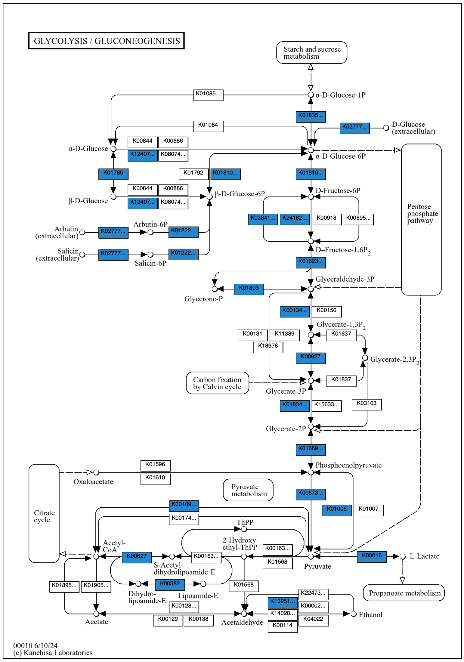
The argument must be a six-digit color hex code, e.g., "#FF0000" for red. A color name, such as red, is refused. It is necessary to enclose a color hex code argument in quotation marks, as # otherwise causes the rest of the command to be ignored as a comment. For a text file with a border column and no value column, these options also take none (see Rings without fills).

The --original-color flag instead uses the original color scheme of the reference map. Global maps are especially colorful, with reactions varying in color across the map as a broad indication of function.

Compare multiple contigs databases

The KO content of multiple contigs databases can be compared. Database file paths can be provided directly on the command line or in an external-genomes text file.

The images in this section show data from contigs databases of genomes from different strains of the same bacterial species.

Color by database

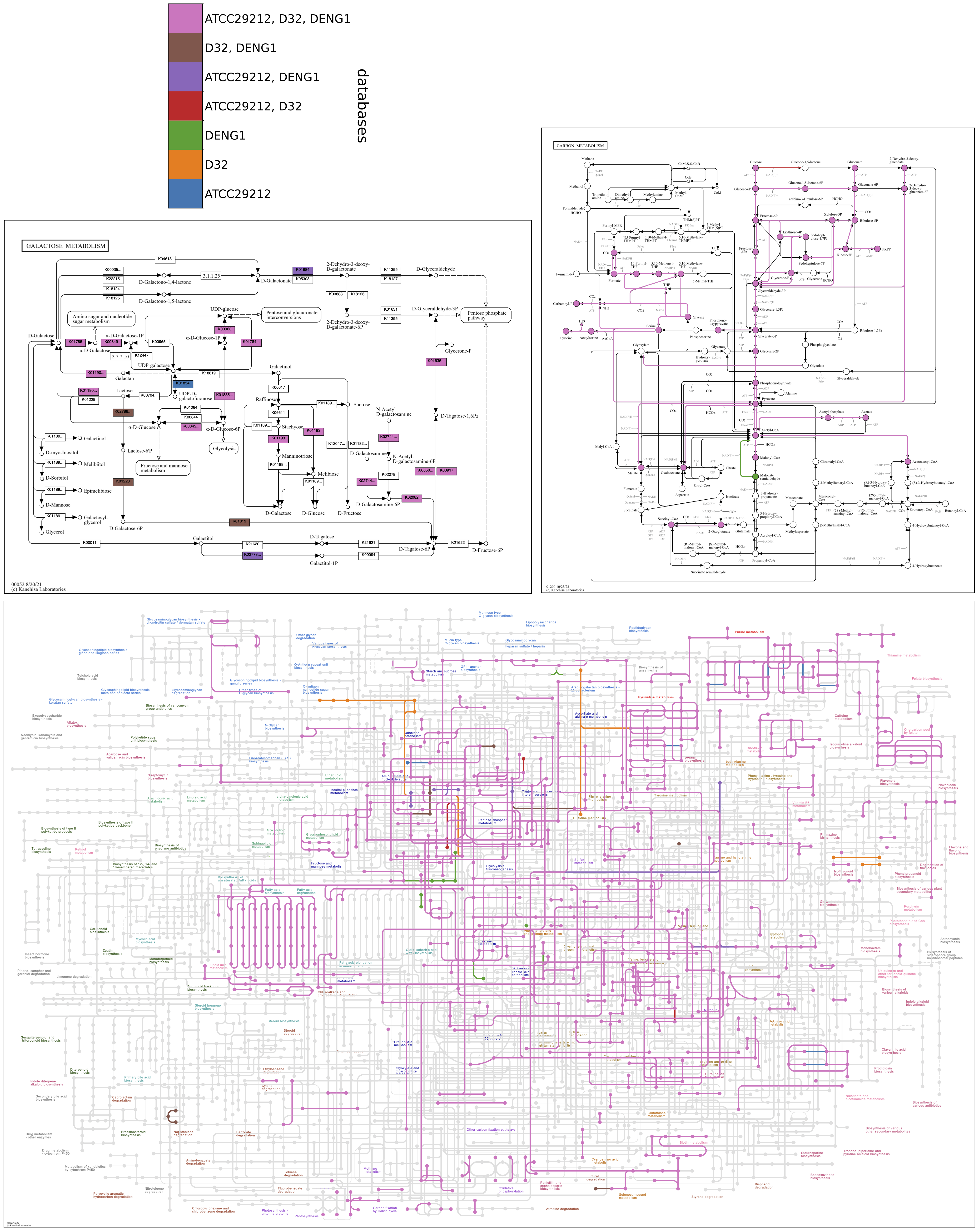
When comparing a small number of contigs databases (realistically, two or three), reactions can be colored by their occurrence across databases, with each color representing a different database or combination of databases. A colorbar key is drawn in a separate file in the output directory, colorbar_reactions.pdf. Each compound circle takes the color of the reaction touching it that is found in the greatest number of databases.

Color by count

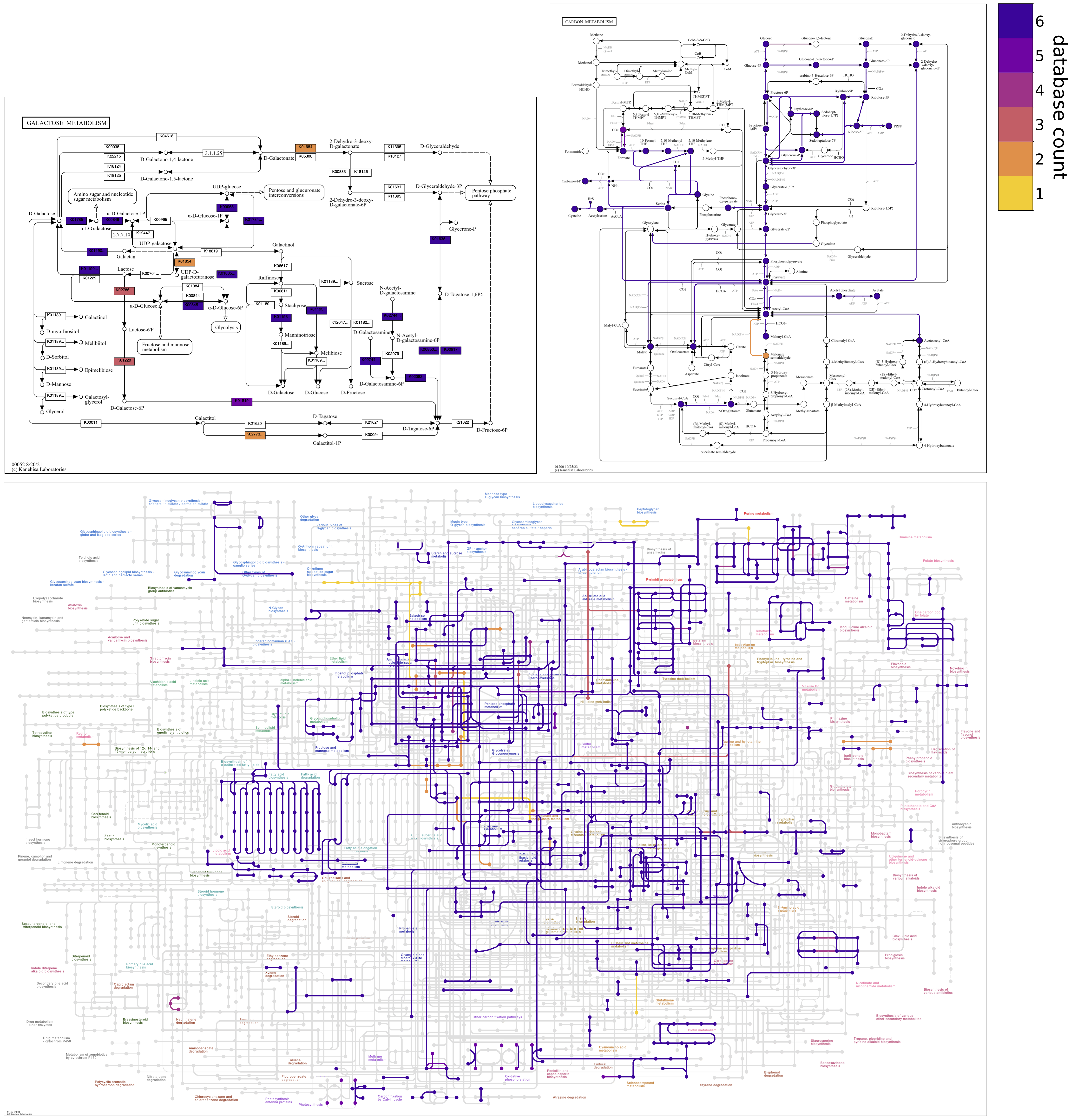
When comparing a larger number of contigs databases, it makes more sense to color reactions by the number of databases in which they occur using a sequential colormap rather than by database or combination of databases using a qualitative colormap. By default, coloring explicitly by database automatically applies to three or fewer databases, whereas coloring by database count applies to four or more databases. The user can override this default with the option, --presence-colormap-scheme, which accepts the values by_membership, by_count, and by_count_continuous. For example, the user may have three databases but wish to color reactions by database count, and so would specify --presence-colormap-scheme by_count.

Counts on a continuous scale

by_count labels one band per count, which asks two things of the colorbar. It needs a distinguishable color for each count. It is refused when the colormap cannot supply that many. A colormap supplies a few hundred distinguishable colors at most. It also needs room to set every one of those labels: a label is sized to fit its band, so past about 40 bands they are too small to read. Asking for by_count above that draws the bands anyway, with a warning that the labels will be tiny.

by_count_continuous colors counts from the same colormap. It draws the colorbar as a gradient rather than as a discrete band per count, so it needs neither a color nor a label per count. It works with any number of samples, contigs databases, genomes, or groups. It is chosen automatically, with a warning, wherever by_count would be refused or its labels would be unreadable.

For a kegg-reaction-txt or kegg-compound-txt file this is the summaries’ count_continuous rather than --presence-colormap-scheme; see Compare samples in an input text file. The count scale of a group’s own maps has the same two choices under its own option, --group-colormap-scheme; see counts in bands or on a gradient.

Where a count scale stops

A count scale runs from 1 to a maximum set by --count-scale-max. observed (the default) stops the scale at the highest count on the drawn maps. total runs it to the number of samples, contigs databases, genomes, or groups being counted. A number sets the maximum. Higher counts take the top color.

This matters for sparse data. With 100 samples and no compound in more than 10 of them, a scale to 100 draws every compound in nearly indistinguishable shades at the bottom of the colormap, while a scale to 10 spreads them across it. The cost of observed is that the scale depends on which maps were drawn, so use total or a number where figures have to be comparable between runs.

Choose the membership colors yourself

Instead of having anvi’o sample a colormap, a color can be given to each sample, contigs database, genome, or group in a kegg-membership-colors-txt file. Pass the file with --reaction-membership-colors. Pass it with --compound-membership-colors for the compound layer of a kegg-compound-txt file. Use this file when each color has to mean the same thing across every figure in a paper.

genome	color
E_faecalis_6240	#1f77b4
E_faecalis_6255	#ff7f0e
E_faecalis_6512	#2ca02c

Coloring by membership colors a reaction by exactly which samples, contigs databases, genomes, or groups contain it, so it needs a color for each combination of them. Each sample, contigs database, genome, or group on its own takes its own color. A combination takes the perceptual blend of its members’ colors. A row naming the combination overrides that blend. The row gives the names in the combination separated by commas. Where the file colors samples, contigs databases, or genomes, the same colors also color the map of each one. A panel of a grid then shows which sample, database, or genome it is. The panel also matches the band of that sample, database, or genome on the unified map. Where the file colors groups, each group’s own maps count that group’s sources. They do not show which of the sources an element is in, so a group’s maps take the group’s color only with --group-colormap tint. That option colors them with a ramp of tints of the group’s color.

Because the colors answer the same question a colormap does, this replaces --reaction-colormap and cannot be combined with it. It also does not apply to coloring by count. A count says how many samples, contigs databases, genomes, or groups contain a reaction, not which ones, so a count has no one sample, database, genome, or group whose color it could take.

Reverse colormap

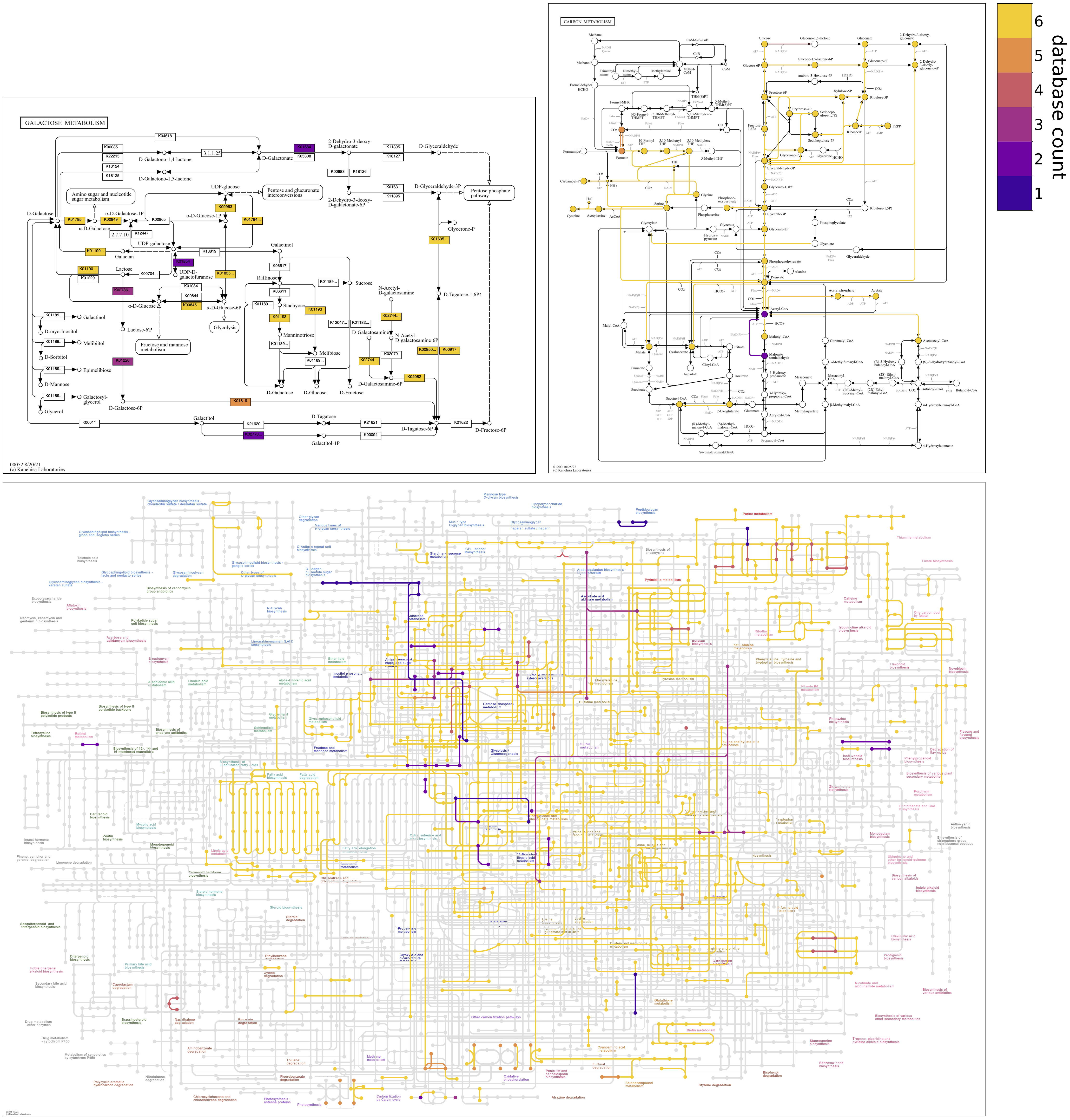
Changing the colormap can draw attention to different information on maps. When coloring by count, the default sequential colormap, plasma_r, goes from dark to light colors; reactions shared among all of the contigs databases are assigned the darkest color, and reactions unique to a single database are assigned the lightest color. The colormap can be reversed to accentuate unshared reactions in the darkest colors and shared reactions in the lightest colors. Reversing the default colormap is accomplished with the option, --reaction-colormap plasma 0.1 0.9. Note that Matplotlib colormap names differing by _r (here, plasma and plasma_r) have the same colors in reverse.

The second and third numerical --reaction-colormap values are not mandatory, but can be provided to trim a fraction of the colormap from each end to eliminate the lightest and darkest colors. The default coloring by database count with plasma_r uses limits of 0.1 0.9. Just changing the colormap (e.g., --reaction-colormap plasma) removes the limits (i.e., changes them to 0.0 1.0), so exactly reversing the default colormap requires that the same limits be specified.

The --reaction-reverse-overlay flag should also be used to reverse the default drawing order. This causes unshared reactions to be rendered above rather than below shared reactions, which is especially important in cluttered global maps.

Show individual database maps

Coloring by count obviously masks the individual contigs databases that contain the different reactions. However, options are provided to enable investigation of the distribution of reactions across databases.

Standalone map files showing the presence/absence of reactions in all of the individual contigs databases can be drawn by using the option, --draw-individual-files, as a flag. Files can be drawn just for a subset of input databases by passing file arguments to the option, e.g., --draw-individual-files contigs_db_1 contigs_db_3. Individual map files for each database are stored in subdirectories of the output directory, with subdirectory names being the project names of databases.

To facilitate comparisons, maps for individual databases can also be drawn alongside the “unified” map containing information from all databases by using the option, --draw-grid, as a flag. Maps for just a subset of individual databases can be shown alongside the unified map in the grid file by passing file arguments to the option, e.g., --draw-grid contigs_db_2 contigs_db_3. Grid files are stored in a subdirectory of the output directory named grid.

The following command would draw individual map files plus grid files for all input contigs databases; a reverse colormap is used in unified maps to emphasize unshared reactions.

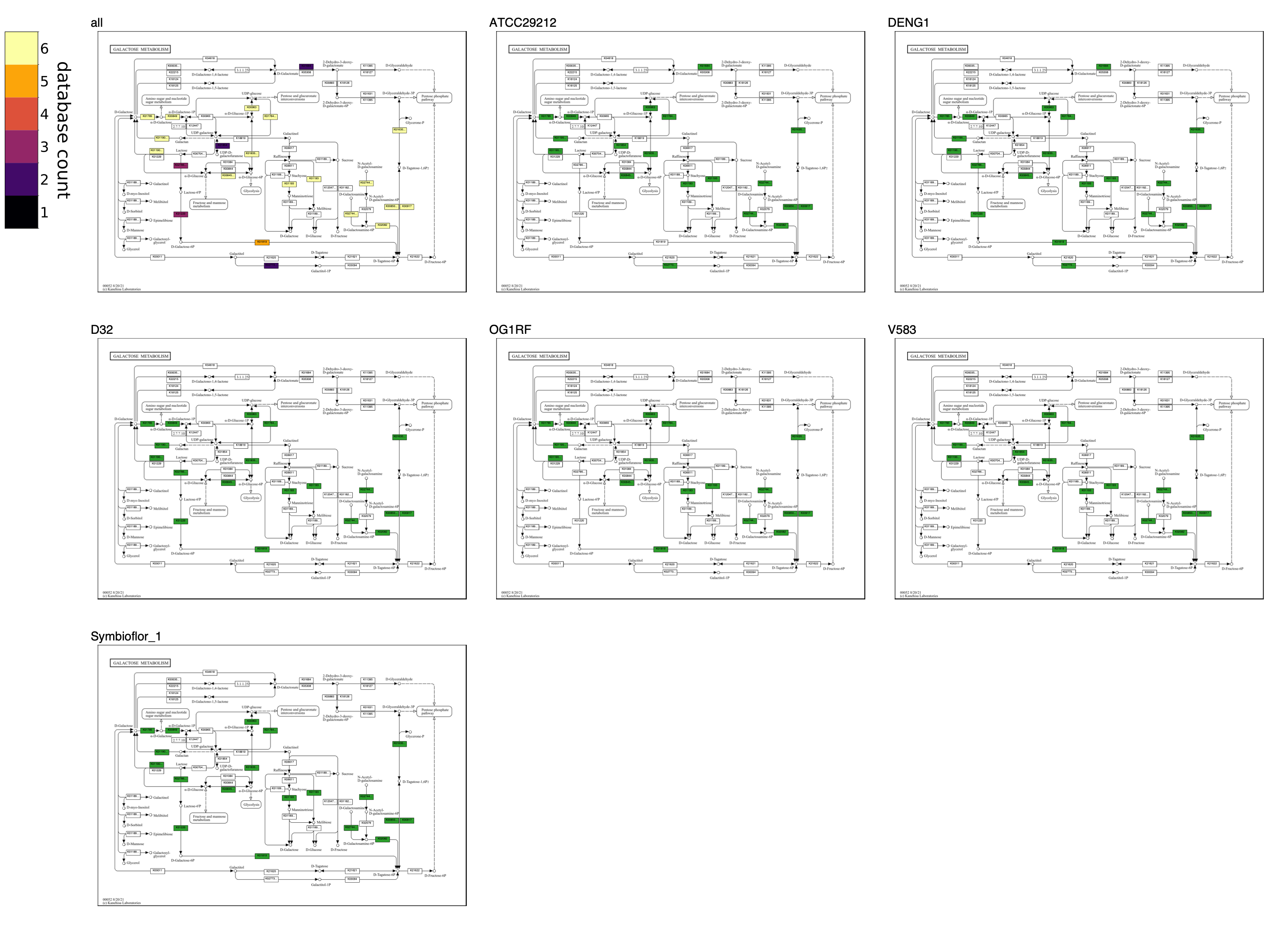
The following map grid uncovers aspects of Galactose metabolism among the genomes of six Enterococcus faecalis strains. The unified map shows that some genomes may be missing steps from Lactose to D-Tagatose-6P in the tagatose-6-phosphate pathway, an alternative to the Leloir pathway for lactose catabolism found in some lactic acid bacteria. The individual maps show that strain ATCC29212 is missing three consecutive steps; OG1RF and V583 are missing two consecutive steps. When sequential reactions catalyzed by different enzymes are missing from a pathway in a closed genomic assembly while present in related genomes, it compellingly suggests that the genes and biological capacity are not in the genome rather than absent due to technical issues of orthology annotation.

Compare groups of contigs databases

A groups-txt file can be supplied to define groups of contigs databases. For example, databases representing genomes could be grouped by taxonomy, databases representing enrichment cultures under different conditions could be grouped by treatment, or databases representing marine metagenomic samples could be grouped by depth. The first column of groups-txt must contain the paths to the input contigs databases provided with --contigs-dbs. The second column headed group must contain group names, such as Pacific, Atlantic, and Arctic. Each database can only be assigned to one group.

A --group-threshold argument between 0 and 1 must also be provided to analyze groups. The group threshold is the proportion of databases in a group that must contain KOs defining a reaction on a map for the reaction to be associated with the group. A threshold of 0 means that ANY database in the group can contain the reaction for the reaction to be considered present in the group. A threshold of 0.75 means that at least 75% of databases in the group must contain the reaction for it to be present. A threshold of 1 means that ALL of the databases in the group must contain the reaction for it be present.

For example, set the threshold to 0.5. Reaction J on a map is defined by KO X and Reaction K is defined by KOs Y and Z. 90% of Pacific, 50% of Atlantic, and 10% of Arctic metagenomes contain KO X, so Reaction J would be colored to indicate that it is found in the Pacific and Atlantic. 0% of Pacific, 15% of Atlantic, and 40% of Arctic metagenomes contain KO Y or KO Z, so Reaction K would not be colored, being considered absent from the groups.

As with comparisons of databases rather than groups, the default setting with two or three groups is to color reactions explicitly by the group or combination of groups in which they occur. With more databases, it makes more sense to color reactions by the number of databases in which they occur using a sequential colormap. The option --presence-colormap-scheme can be used to override this behavior, e.g., to color reactions by group count rather than explicitly by membership using --presence-colormap-scheme by_count.

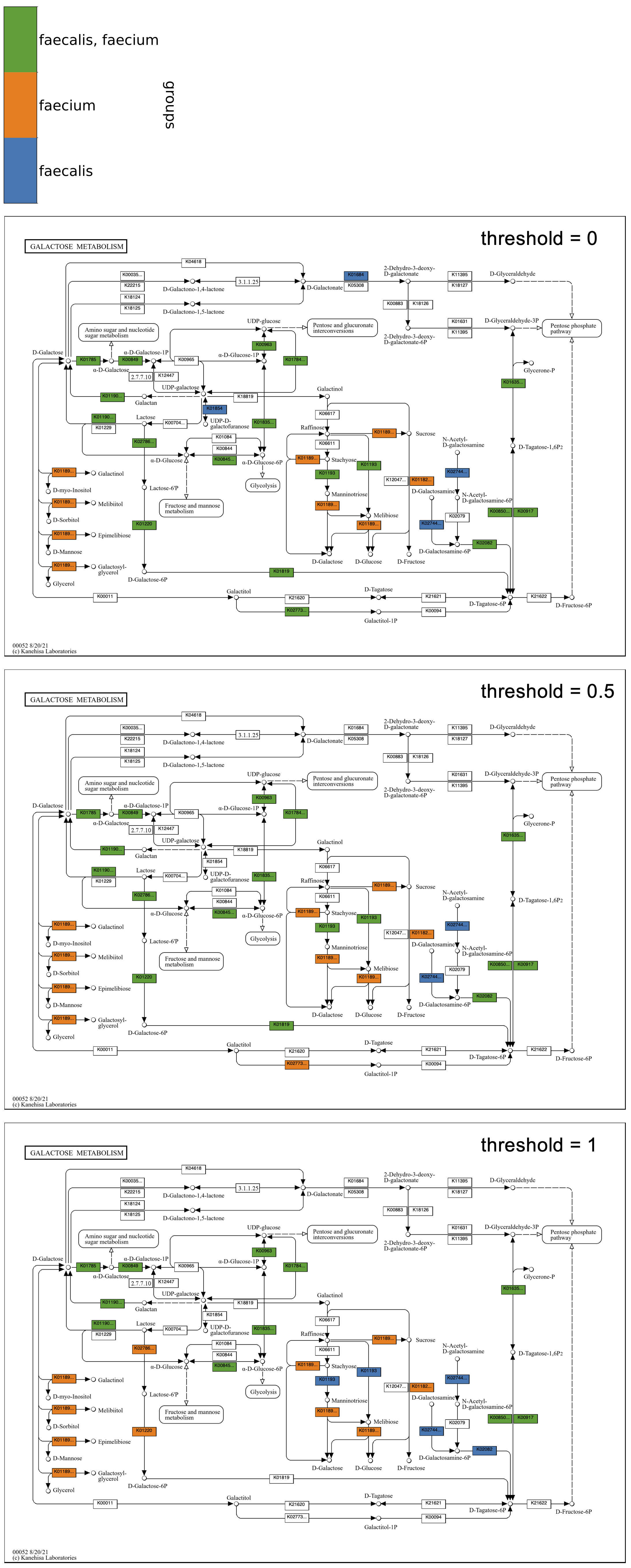
The following example continues with Galactose metabolism, now including two groups of genomic contigs databases from Enterococcus faecalis and Enterococcus faecium. The program was run three times with different values of --group-threshold. The top map has a threshold of 0, so a reaction is included in the faecalis group if it has corresponding KOs in any of the six faecalis genomes, and included in the faecium group if it has KOs in any of the five faecium genomes. The middle map has a threshold of 0.5, so reactions in the faecalis group must be in at least four of six faecalis genomes, and reactions in the faecium group must be in at least three of five genomes. The bottom map has a threshold of 1. As in the map grid of faecalis genomes from above, the group maps show that some faecalis strains may be missing steps from Lactose to D-Tagatose-6P in the tagatose-6-phosphate pathway, though at least four of the strains have each step. In comparison, a greater proportion of the faecium strains have these steps, with all of them having the first two, as seen in the bottom map with a threshold of 1.

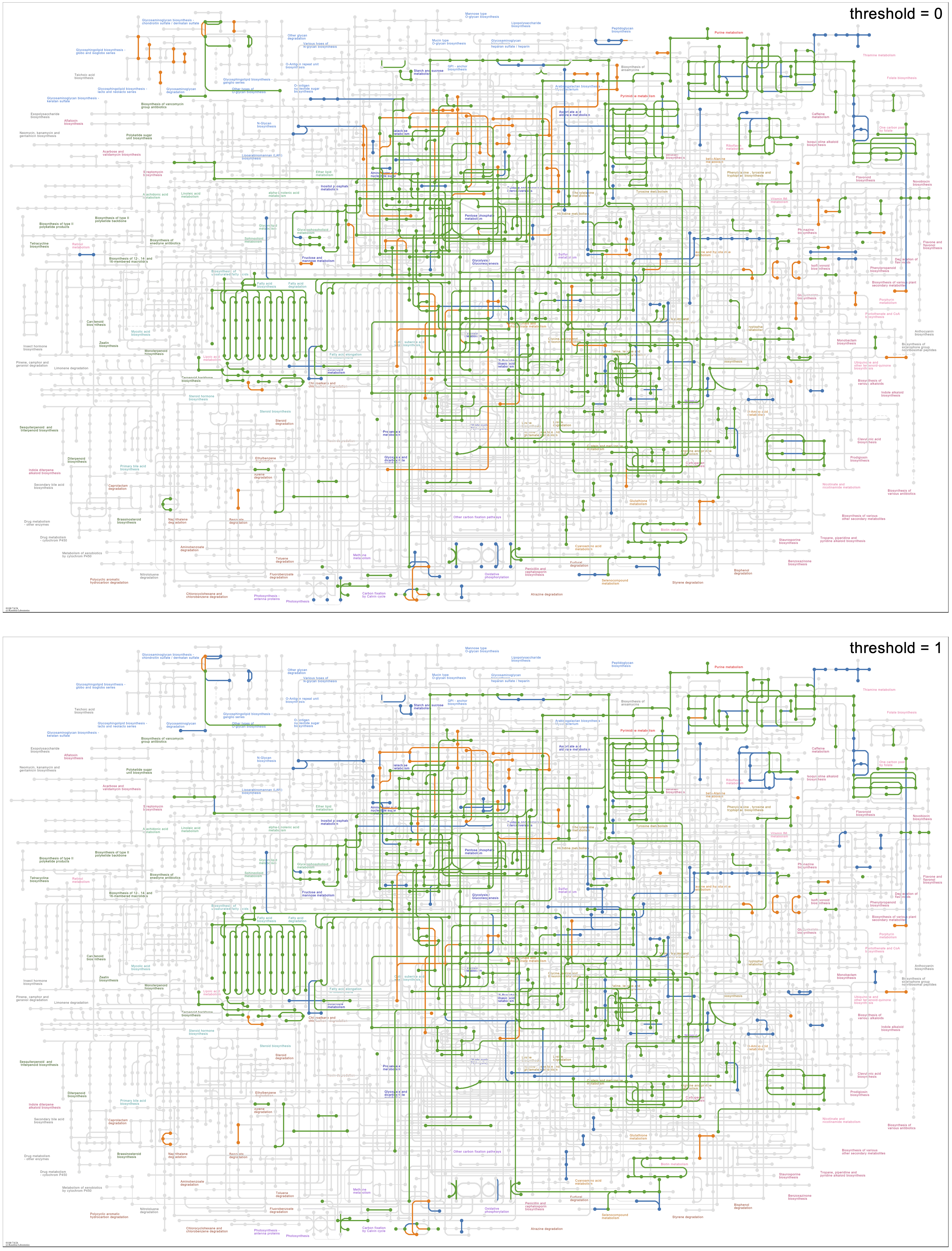
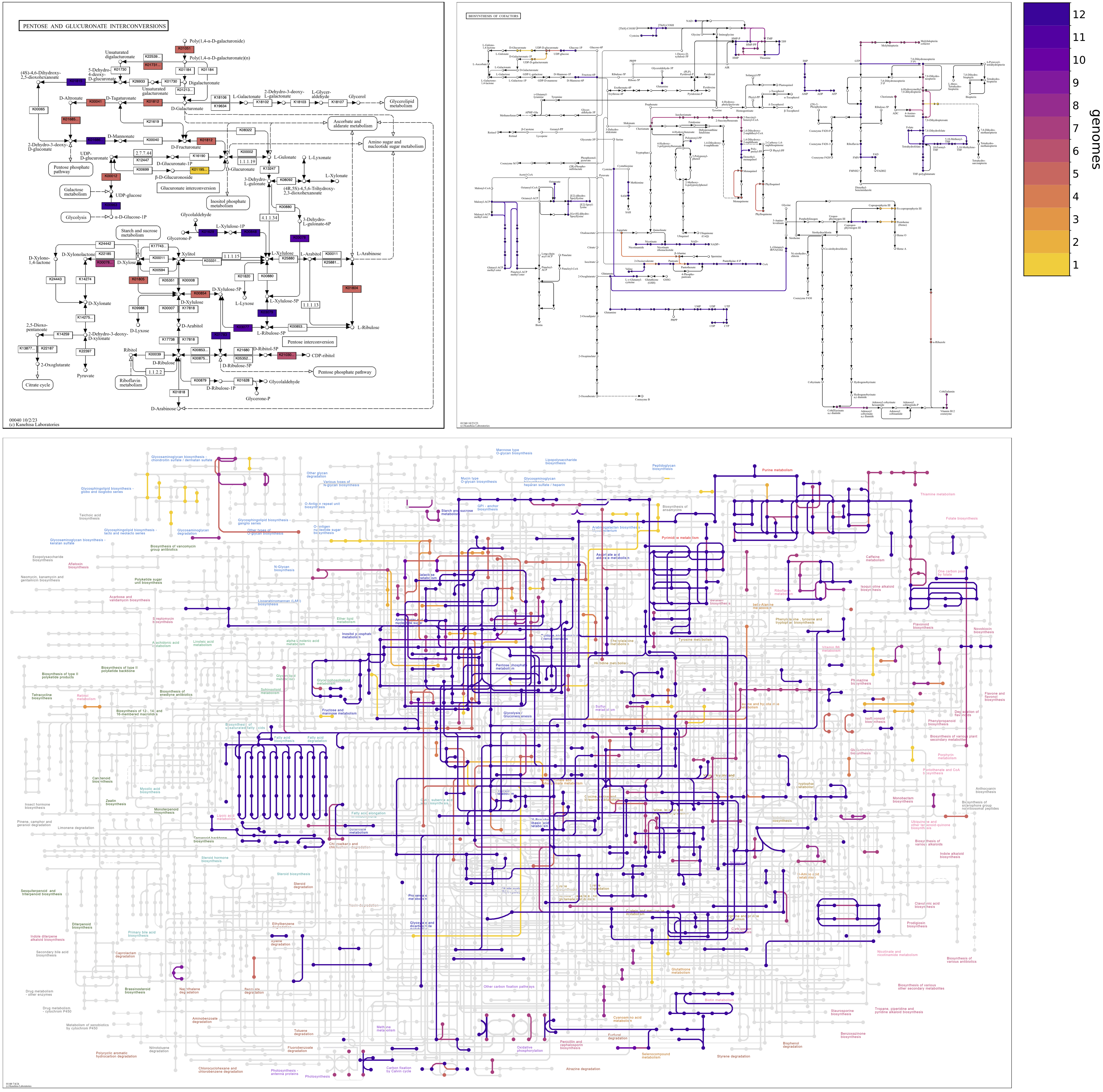
Below is the Global metabolism map using the same species groups with thresholds of 0 and 1. The map with a threshold of 0 shows how some metabolic pathways are present only in faecalis or faecium genomes, and the threshold of 1 shows how some of these unique pathways are conserved amongst all of the genomes of the species, such as the faecalis (blue) reactions in the upper right corner of the map involved in cofactor biosynthesis, and the faecium (orange) reactions in the upper center involved in sugar metabolism, including galactose, pentoses, and uronates.

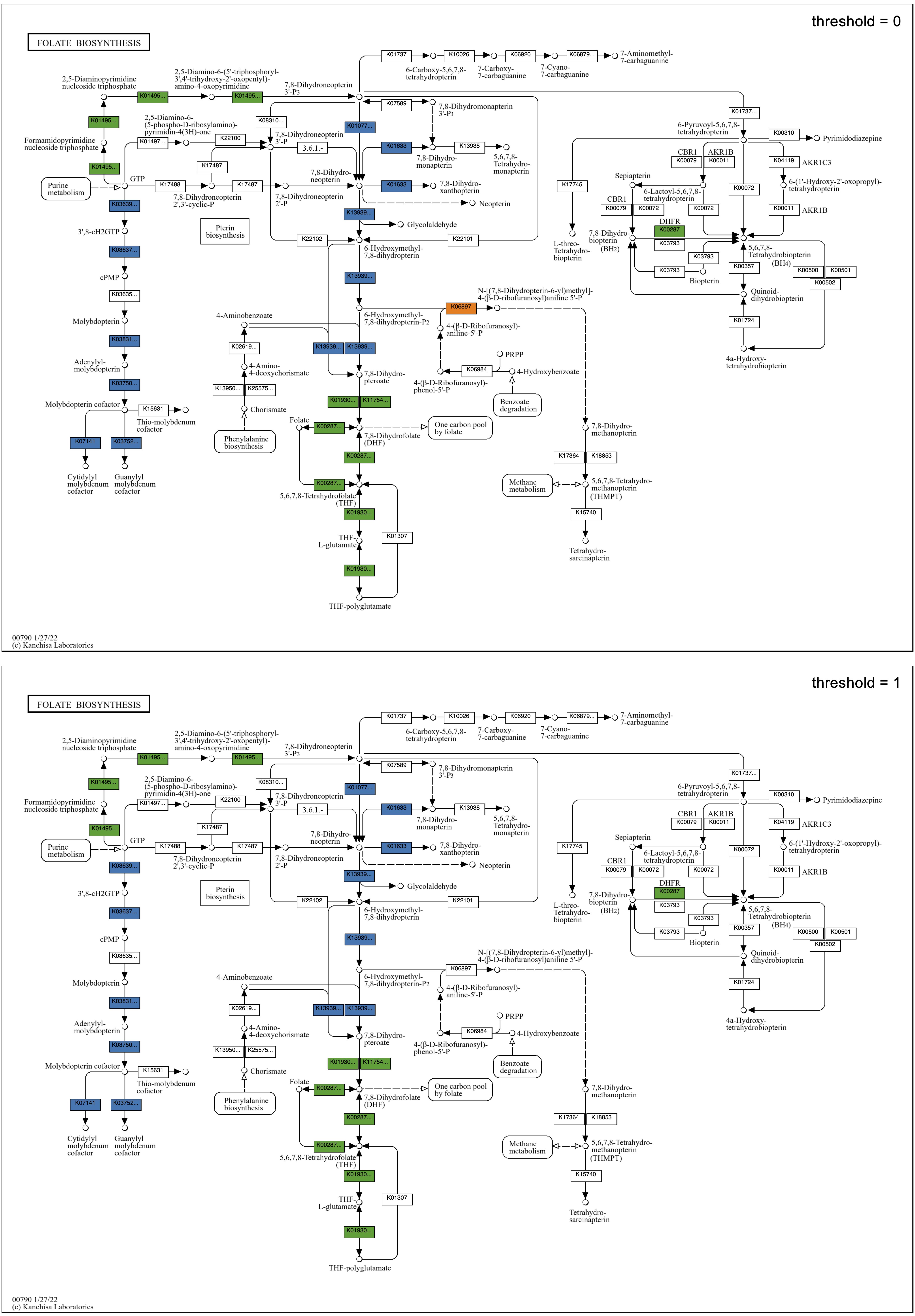
Exploring the Folate biosynthesis map given the observation regarding cofactors in the global map, all faecalis genomes have a full set of enzymes required for folate biosynthesis, whereas all faecium genomes appear to be missing a big chunk of the pathway in the center of the map, from 7,8-Dihydroneopterin 3'-3P to 7,8-Dihydropteroate. The implication of folate auxotropy in faecium is confirmed by Ramsey, Hartke, and Huycke in The Physiology and Metabolism of Enterococci: “Characteristically, E. faecium requires folate while E. faecalis does not.”

Show individual group maps

Maps can be drawn for individual groups as grids or separate files. These depict the occurrence of reactions across contigs databases in each group, identical to the maps that can be drawn to compare ungrouped databases.

Coloring options are available for individual group maps, --group-colormap, --group-colormap-scheme and --group-reverse-overlay. Unlike drawing maps for ungrouped databases, drawing maps for individual groups always colors reactions by database count regardless of the number of databases in the group in order to facilitate the comparison of individual group maps using the same colormap scheme.

With the option, --draw-individual-files, individual group map files and a colorbar file are written to subdirectories of the output directory named after groups. With the option, --draw-grid, map grid files and colorbar files are written to the grid subdirectory of the output directory. There are colorbar files for each individual group in the grids: using our example Enterococcus dataset, there are files like colorbar_faecalis.pdf and colorbar_faecium.pdf.

A subset of groups can be considered, limiting the individual files drawn or the individual maps shown in grids to the specified groups, e.g., --draw-individual-files faecalis, --draw-grid faecium.

The following command would draw individual map files plus grid files for all groups. A reverse colormap is used in individual group maps to emphasize reactions that are not shared across databases of the group. The group threshold is set to 0, meaning a reaction is classified in a group if it occurs in any database, since the individual group maps reveal the number of databases in which the reaction occurs.

Give each group’s maps its own color

A group’s own maps show a magnitude — the number of the group’s databases, genomes, or samples containing a reaction — while a group’s color on the unified map is an identity. The two are separate by default: --group-colormap names a colormap engineered for showing magnitude, and a kegg-membership-colors-txt file does not change it.

To give each group’s maps the group’s own color, give --group-colormap tint. Each group’s scale is then a ramp running from a pale tint to that group’s own color, so faecalis panels are drawn in shades of one hue and faecium panels in shades of another. Every group’s ramp is built the same way, so the panels of a grid stay comparable while each says which group it is.

The two decimal values --group-colormap also accepts then say how far from white each ramp starts and stops rather than which fraction of a colormap to use, defaulting to 0.25 1.0. The pale end stops short of white on purpose: standard and overview maps keep white for their own unhighlighted elements, so a ramp reaching it could not be drawn there. Anvi’o checks every group’s ramp against those reserved colors before writing any file, and if one collides it says to start the ramp further from white — that is, to raise the first of the two values.

Since one scale styles every layer’s group maps at once, a run whose reaction and compound layers give the same group different colors is refused; pointing both --reaction-membership-colors and --compound-membership-colors at a single file is the simplest way to keep them in step.

Counts in bands or on a gradient

A group’s count scale is drawn in discrete bands, one per count the scale runs over — which is where --count-scale-max stops it, not how many sources the group has — or as a gradient over that same range. These are the two choices --presence-colormap-scheme gives the unified map, under --group-colormap-scheme:

Which color a count takes is the same either way: it is always sampled at an even fraction of the group’s colormap or ramp, so this option changes the colorbar and nothing on the maps themselves. by_count needs a distinguishable color for every count and room to label every band, both of which a group of many sources can exhaust; by_count_continuous needs neither, since a color on a gradient reads as a position along the range of counts rather than as an exact count, and so works for a group of any size. By default the bands are drawn while they can be told apart and read, and the gradient takes over with a warning where they cannot — see counts on a continuous scale.

Unlike --presence-colormap-scheme, which each layer sets for itself, one scheme covers every layer’s group maps, because the reaction and compound layers of a group’s map share one set of colors and one colorbar. For the same reason the choice is made once for the whole run rather than per group, so that the panels of a grid all carry the same kind of colorbar. There is no by_membership here: a group’s own map counts that group’s sources and never shows which of them contain an element.

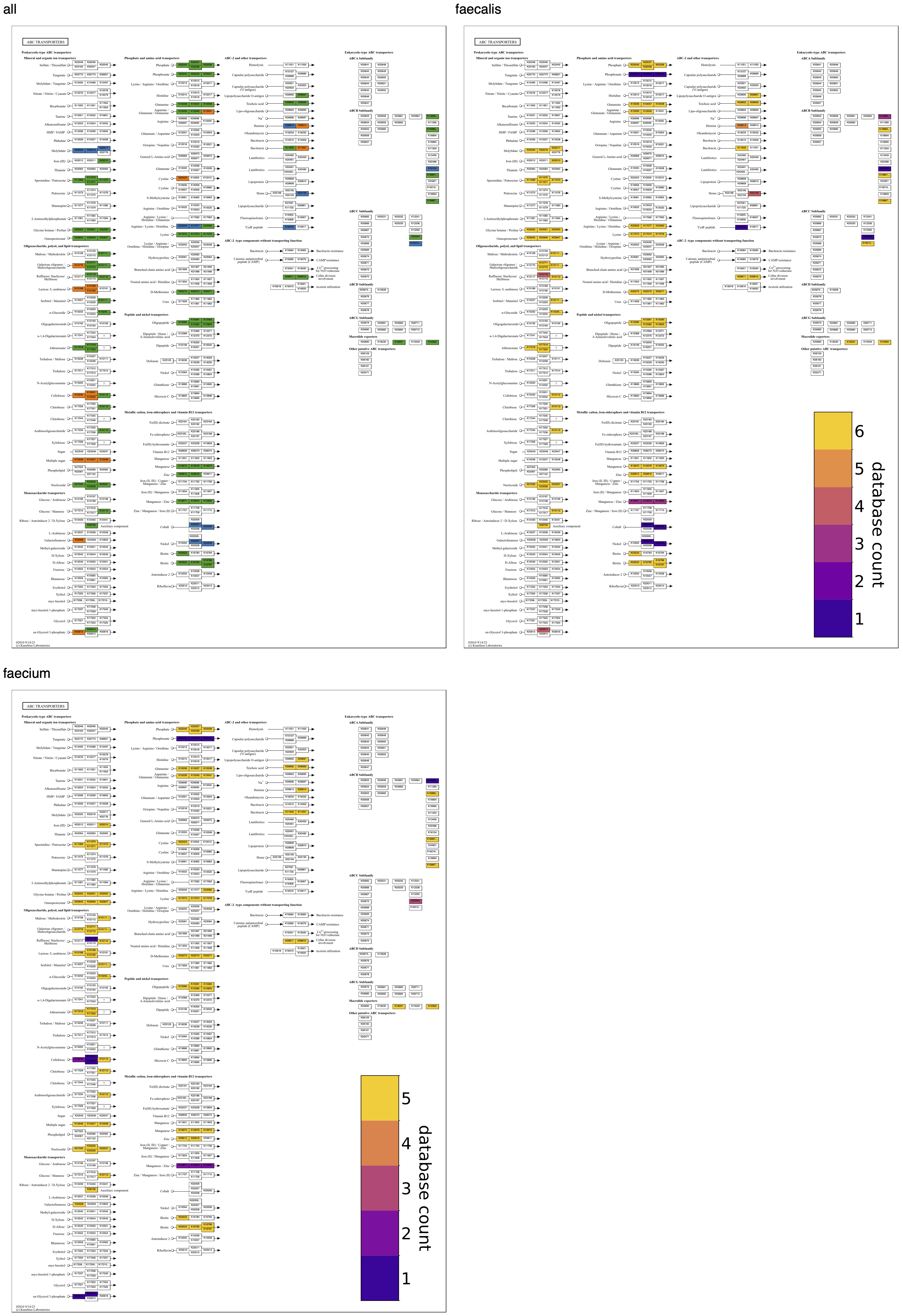
Continuing with the comparison of Enterococcus species, the Folate biosynthesis map from above shows, on the left side, that all faecalis genomes have the pathway for molybdenum cofactor (MoCo) biosynthesis, unlike any faecium genomes. A molybdenum requirement in faecalis but not faecium is supported by the annotation of a molybdate transporter in all faecalis genomes and no faecium genomes, as seen in an ABC transporters map grid – in the map of “all” groups, it is the top transporter colored blue in the first column.

Compare samples in an input text file

The kegg-reaction-txt and kegg-compound-txt files introduced above can compare data across origins in the same way as multiple contigs databases, without any anvi’o database. Add a sample column that assigns each row to its sample of origin, where a sample can be, for example, a genome (e.g., E. coli versus K. pneumoniae), a metagenome, or a transcriptomic, proteomic, or metabolomic sample. Every row must have a sample.

When a layer’s file has a sample column but no value column, its elements are compared across samples just as reactions are across contigs databases: they are colored by the sample or by the number of samples in which they occur, a colorbar_reactions.pdf (and, for the compound layer, colorbar_compounds.pdf) key is written, and all of the same coloring and output options apply, including --reaction-colormap, --compound-colormap, --reaction-reverse-overlay, --draw-individual-files, and --draw-grid. Whether elements are colored by which samples or by how many is set per layer with --reaction-sample-summary/--compound-sample-summary (membership, count or count_continuous; by default membership for 3 or fewer samples, count above that, and count_continuous where a discrete scale would run out of distinguishable colors or of room to label its bands). count writes a discrete colorbar with one band per count and count_continuous writes a gradient from the lowest count to the highest, as described under counts on a continuous scale. These per-layer options take the place of --presence-colormap-scheme, which applies to contigs database and pangenome inputs only and is rejected for a text run. (If a file has a value column, that value colors each sample’s own map; see Color elements by a quantitative value.)

When elements are colored by which samples or groups contain them, the color of each of them can be given explicitly in a kegg-membership-colors-txt file rather than sampled from a colormap — --reaction-membership-colors for the reaction layer and --compound-membership-colors for the compound layer, each taking the place of that layer’s colormap. See Choose the membership colors yourself. The file works the same way here as it does for contigs databases and genomes. Without a groups-txt, the map of each sample of a layer with a value column shows that sample’s values, so the file colors only the unified map.

Samples can be grouped with a groups-txt file, like contigs databases. The file has the same format, but the items in its first column must be the sample names from the sample column. The two files share one sample space and one groups-txt. Whenever a layer summarizes its groups by presence — the default — --group-threshold must accompany --groups-txt, as with contigs databases: it sets the proportion of a group’s samples in which an element must occur for the group to be considered to contain it.

Pangenomic database

Pangenomes are treated similarly to multiple contigs databases. Rather than comparing the distribution of KOs across contigs databases, KOs assigned to pan-db gene clusters are compared across genomes. Here is the basic structure of the command.

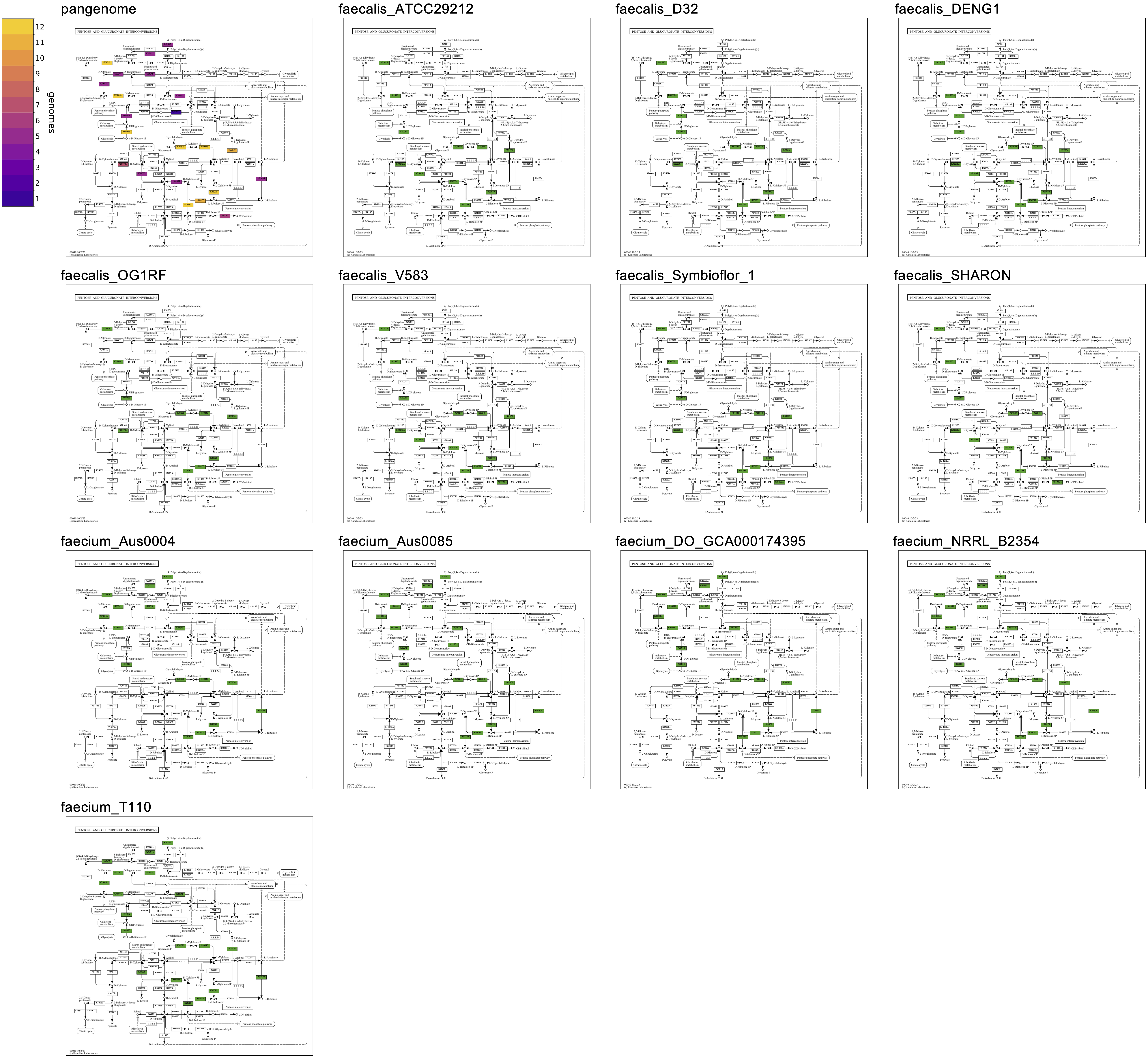
The following maps were produced with the basic command structure for a pangenome of seven Enterococcus faecalis and five Enterococcus faecium genomes. A metagenome-assembled genome (MAG) has been added to the set of E. faecalis genomes from above.

Genomes defined in the pangenomic database can be grouped like contigs databases. The groups-txt file has the same format, but the items in the first column must now be the names of the genomes in the pangenome rather than contigs database files. The following command colors reactions by group, assigning a reaction to a group if the reaction is in at least 50% of the group’s genomes.

All of the options demonstrated in comparing contigs databases apply to pangenomes as well, including drawing map grids and changing the colormap to emphasize reactions unshared between genomes.

Continuing with the Enterococcus pangenome, the following map grid shows differences in Pentose and glucuronate interconversions between faecalis and faecium and between strains of each species. faecalis genomes are enriched in genes for xylose metabolism (towards the bottom of the map), and faecium genomes are enriched in enzymes for uronate metabolism (toward the top of the map). The faecalis MAG, SHARON, has genes for the catabolism of Xylose, via D-Xylulose and D-Xylulose-5P. These are also annotated in three of the faecalis isolate genomes, ATCC29212, DENG1, and V583, but not the other three, D32, OG1RF, and Symbioflor_1. Xylose utilization is known to be variable among faecalis strains.

Consensus KOs

The functional annotations of gene clusters as a whole are imputed to the genes in the cluster. The method of assigning consensus annotations to a cluster is parameterized by the options, --consensus-threshold and --discard-ties. By default, the consensus threshold is 0 and ties are not discarded. The consensus threshold sets the proportion of genes in the cluster that must have the same functional annotation to be assigned to the cluster as a whole, so a value of 0 means that the most abundant annotation is used regardless of its abundance. To discard ties means to ignore candidate consensus annotations that are equally abundant among genes. The default behavior randomly breaks ties. The consensus KO of a gene cluster becomes the KO annotation of all the genes in the cluster for the purposes of analysis.

Color elements by a quantitative value

The sections above color elements to show presence/absence. A layer can instead be colored by a continuous quantitative value simply by including a numeric value column in its kegg-reaction-txt or kegg-compound-txt file. The single column that is not a key column — accession; sample; in the reaction file, gene_id — is auto-detected as the value column, and its header labels the colorbar. The column can have any name. A column named by --reaction-slice-weights, --reaction-border-column, or --compound-border-column is left out of this detection. Uses can include coloring reactions by gene, transcript, or protein levels in a kegg-reaction-txt file, and compound levels in a kegg-compound-txt file. Every row must have a numeric value.

For a reaction file of KO accessions, the value of a KO is the aggregate of its optional gene rows’ values, and KO accessions are aggregated to map element values. Two options set these, both defaulting to sum: --reaction-gene-aggregation combines the genes carrying one KO into that KO’s value, and --reaction-accession-aggregation combines the KOs of one map element into that element’s value. They can differ — averaging across the genes of each KO while totaling across the KOs of a reaction, for instance. The compound layer has only the second of the two, --compound-accession-aggregation, since a compound file names no genes and no two of its rows may name the same compound in the same sample. Accession aggregations reduce values within a sample.

The reaction layer and the compound layer are colored on independent scales, each through its own sequential colormap and each getting its own continuous key: colorbar_reactions.pdf and colorbar_compounds.pdf. A border column takes keys of its own, such as colorbar_reactions_border.pdf. The reaction colormap is set with --reaction-colormap and the compound colormap with --compound-colormap (both default plasma_r). The drawing order of overlapping elements can be flipped per layer with --reaction-reverse-overlay and --compound-reverse-overlay.

If a layer’s file has a sample column, the value column colors each sample’s own magnitude: maps for individual samples are added with --draw-individual-files and/or --draw-grid, as when comparing samples by presence/absence, and they share a single colorbar_reactions_samples.pdf and colorbar_compounds_samples.pdf so their colors are directly comparable across samples. That makes two scales per layer, the unified map’s and the one those individual maps share. They are colored by the layer’s one colormap from --reaction-colormap/--compound-colormap unless --reaction-individual-colormap/--compound-individual-colormap gives the individual maps a distinct colormap; see Give the two scales different colormaps. A border column adds two scales of its own, keyed in colorbar_reactions_border.pdf and colorbar_reactions_border_samples.pdf for the reaction layer.

Summarize samples and groups

A layer with a sample column involves multiple separate reductions, and each has its own option:

Level	Option	What it reduces
genes of an accession	--reaction-gene-aggregation (an aggregation; sum by default; or a rule for categorical values)	the genes carrying one KO or KEGG reaction accession → that accession’s value. With --reaction-slice-by gene, each gene keeps its own value, and this option is refused.
accessions of an element	--reaction-accession-aggregation/--compound-accession-aggregation (an aggregation; sum by default; or a rule for categorical values)	the constituent accessions of a map element → that element’s value. With --reaction-slice-by accession, each slice keeps the value of its own accession instead. With --reaction-slice-by gene, the rows of one gene for the accessions of an element → that gene’s value, with mean as the default. An aggregation that changes a single value, such as std, is then refused.
across samples	--reaction-sample-summary/--compound-sample-summary (count, count_continuous, membership, an aggregation, or a rule for categorical values)	a set of samples → one value or one presence value per map element, or per slice with --reaction-slice-by
across groups	--reaction-group-summary/--compound-group-summary (count, count_continuous, membership, an aggregation, or a rule for categorical values)	the groups of a groups-txt → one value or one presence value per map element, or per slice with --reaction-slice-by
weights of the genes of an accession	--reaction-slice-weight-aggregation (sum by default, or mean)	the weights of the genes carrying one accession → that accession’s weight, which sizes its slice. This applies only where --reaction-slice-by accession slices the elements or --reaction-border-slice-by accession slices the rings.
shares across samples and groups	--reaction-slice-share-summary (share_mean by default, or pooled_sum)	the shares of a slice in a set of samples, or in the groups → its share on the map of a group or the unified map

A border column has its own versions of the first four options: --reaction-border-gene-aggregation, --reaction-border-accession-aggregation/--compound-border-accession-aggregation, --reaction-border-sample-summary/--compound-border-sample-summary, and --reaction-border-group-summary/--compound-border-group-summary. They reduce the values of the border column, and their defaults differ from those of the fill (see Color borders by a second column). The last two rows also size and pool the slices of rings that are divided on their own (see Slice rings).

An aggregation is sum (default), mean, max, min, median, std — or any other unsuggested pandas aggregation that reduces a series of numbers to one number, such as var or sem. Names that transform rather than reduce (cumsum) or that only a grouping offers (first) are rejected. Where an aggregation is undefined for the values available, as std is for a single value, the affected elements are left uncolored. circular_mean averages values that repeat after a period, such as clock times, and requires --reaction-value-period/--compound-value-period (see Color clock times with a cyclic colormap). angular_deviation measures how far such values are spread apart, on the unified map only.

A summary pools the values of a map element, not of an accession. An element’s value in a sample is the aggregate of its accessions in that sample. Without --reaction-element-normalization/--compound-element-normalization, this is the value that the sample’s own map draws, so the sample summary pools what the maps of the individual samples show. With groups, the group summary then pools the values of the groups.

With --reaction-slice-by, a summary pools the values of each slice instead. A slice’s value in a sample is the value of its one accession or gene, so the summary pools the values of that accession or gene across the samples or groups. The last two rows of the table apply only to slices sized by --reaction-slice-weights, of elements or of rings. See Draw elements in slices.

The sample summary drives the unified map when there are no groups, and each per-group map (produced when using --draw-individual-files or --draw-grid) when there are. The group summary colors the unified map when there are groups.

Note that with groups, the per-group map either shows the count of that group’s sample — the default case — or, with a --reaction-sample-summary/--compound-sample-summary aggregation argument, the samples’ pooled value; --*-sample-summary is therefore not permitted with a presence name (count, count_continuous or membership) when using groups. Whether that count is drawn in bands or on a gradient is set for every layer’s group maps at once by --group-colormap-scheme, not per layer; see counts in bands or on a gradient. For categorical values, a rule given to --reaction-sample-summary/--compound-sample-summary colors each group’s map by the value that it chooses among the group’s samples.

Both summaries default to presence: in how many (count and count_continuous) or exactly which (membership) samples or groups an element occurs. membership is chosen automatically for 3 or fewer samples or groups, and count is chosen above that. This matches the presence/absence behavior for contigs databases and genomes. Where a discrete scale would run out of distinguishable colors or of room to label its bands, count_continuous is chosen instead. A warning says so. count draws a discrete colorbar with one band per count, while count_continuous draws a gradient from the lowest count to the highest — see counts on a continuous scale. Presence is the default because it is meaningful for any set of samples, whereas pooling values is only meaningful when the samples are commensurable: averaging the coverages or concentrations of replicates of one condition makes sense, while pooling them across unrelated conditions does not. Name an aggregation to pool values instead, which draws a continuous colorbar for that view; std across replicate samples turns the map into a picture of where they disagree. Note that count, count_continuous and membership always mean presence at these two levels, so pandas count (a row count) is not reachable through a summary option — use it with --reaction-gene-aggregation if you want it. The summaries of a border column, such as --reaction-border-sample-summary, have no default and refuse presence names, since the fill already shows presence.

The sample and group summaries in the unified maps both default to presence, even with a quantitative value column. The default is membership for 3 or fewer samples or groups, count above that, and count_continuous beyond what the colormap can distinguish. Presence is the default because it is meaningful across any set of samples. Pooling values is only meaningful for commensurable samples. For example, it makes sense to average transcript abundances across samples from replicate conditions, but not from unrelated conditions. Pooling values across samples is triggered by providing an aggregation argument to --reaction-sample-summary/--compound-sample-summary or --reaction-group-summary/--compound-group-summary. std at sample and group levels map how much samples and groups disagree. Note that count, count_continuous and membership always mean presence at these two levels, so pandas count (a row count) is not reachable through a summary option, but may be used through gene and accession aggregation options, say for drawing counts of the number of genes per reaction. The summaries of a border column, --reaction-border-sample-summary/--compound-border-sample-summary and --reaction-border-group-summary/--compound-border-group-summary, do not default to presence. Without one, the unified map shows no border.

A layer can show presence in the overview and values per sample or group. With the default presence summary, the unified map gets a colorbar of sample or group counts or memberships, while per-sample maps keep a continuous colorbar. The sample and group levels can be treated independently — replicate samples can be averaged within each condition (group) while the unified map summarizing all conditions shows in how many conditions each element occurs, with a group containing an element when at least half of its samples do:

Limit the color scale

By default a continuous scale spans exactly the values it is given, from the lowest map element to the highest. A handful of extreme elements can therefore stretch the colors over a range in which everything else is crowded into one end and cannot be told apart. The --reaction-value-limits and --compound-value-limits options bound the scale so that this cannot happen. Each option takes two values, a minimum and then a maximum. Either can be the word none to leave that end wherever the data puts it.

A limit sets that end of the scale, whether or not any value reaches it. Given the limits above, the scale runs from -6 up to the highest value. Every element below -6 is drawn in the color at the bottom of the scale. Where values lie past a limit, its label is marked ≥ or ≤: the color there stands for that value or anything beyond it. A scale whose values all stay above -6 still starts at -6.

Limits are read in the units of the colorbar, which are the values of map elements after both reductions — gene to accession (optional) and accession to map element — have been applied. With a sample column, the unified map shows a summary of these element values across the samples or groups. With the default sum at the accession level, an element standing for a dozen KOs may sit well past any single value in the file, so limits should be chosen against the scale that is actually drawn rather than against the input column. With --reaction-slice-by, the colorbar shows the values of slices instead, each the value of one accession or gene, so limits are read in those values.

A layer with a sample column has two continuous scales, and each is limited separately: --reaction-value-limits bounds the unified map’s scale, while --reaction-individual-value-limits bounds the single scale shared by the per-sample maps (or the per-group maps given a groups-txt). The two are kept apart because a summary can put them on quite different footings — for example, the mean across samples clusters more tightly than the per-sample values behind it — so limits that suit one can be inappropriate for the other. Setting only one of the two is perfectly legitimate, and anvi’o warns when you do, since the scale left alone goes on spanning whatever its own values reach.

The compound layer takes the same pair, --compound-value-limits and --compound-individual-value-limits, on its own independent scale.

Note that these options are a different thing from the two decimals --reaction-colormap/--compound-colormap accept, which choose what fraction of the colormap to sample and say nothing at all about the values.

Center the color scale

A diverging colormap, such as ‘RdYlGn’ or ‘RdYlBu_r’, has a neutral color at its middle and two opposed ramps either side. That middle color only means something if the scale puts it where the value it stands for actually is, and by default a scale spans exactly the values it is given: a column of log ratios running from -2 to +6 puts the neutral color at +2, and paints the negatives in the same half of the colormap as some positives.

--reaction-value-center and --compound-value-center put a value at the middle of the scale instead. Used as a bare flag, each centers the scale on 0; give it a number to center the scale on that number instead.

The scale is widened, never narrowed. It comes to run the same distance either side of the center, reaching as far as the farther of its two ends already did: values from -2 to +6 centered on 0 give a scale from -6 to +6. Nothing is clipped that was not clipped before, and the scale stays linear, so the same distance in color goes on meaning the same distance in value on both sides of the center. The colorbar is ticked at the center, wherever it falls, so a reader can see where the middle of the scale is.

The price of that is the shorter side of the colormap going partly unused — the honest picture of values that lean one way. To fill the colormap again, trim the longer side: --reaction-value-limits none 2 along with the centering gives a scale from -2 to +2 whose top is marked ≥ 2.

Limits and a center act on a scale in that order. The limits set their ends of the scale, and the center then widens whichever side falls short. The two can therefore conflict. Centering never moves a limit. Where it would have to, anvi’o refuses. It does not quietly undo the limit. A center lying outside its own scale’s limits, or on one of them, is refused as well.

A layer with a sample column has two scales here as well, centered separately: --reaction-value-center centers the unified map’s, and --reaction-individual-value-center the one shared by the per-sample (or per-group) maps. Centering only one of the two earns a warning, because unless --reaction-individual-colormap (described in the next section) gives them each a colormap, one colormap colors both, and its middle color would then mean the centered value on the one map and whatever the values happen to leave in the middle on the other.

Centering says nothing to a reader looking at a sequential colormap, which has no middle to speak of, so anvi’o warns when a centered scale is drawn from one — the default plasma_r included. It also warns when a diverging colormap has been trimmed off-center by the two decimals accepted by a colormap option such as --reaction-colormap, since the neutral color is then no longer in the middle of what is drawn.

Give the two scales different colormaps

The unified and per-sample/per-group scales are on one colormap by default, which can work when they show the same quantity, such as the values of one sample beside the mean of them all. The different types of maps can also show quantities of different kinds, and then a single colormap invites mistaking one scale for the other. For example, with --reaction-sample-summary std, the unified map shows how much replicate samples disagree, a spread that is never negative and is not measured equivalently to the underlying values shown in the per-sample maps, which may include negative numbers.

--reaction-individual-colormap gives the per-sample or per-group scale a colormap of its own, leaving --reaction-colormap to the unified map. The argument structure is the same as --reaction-colormap, a colormap name optionally followed by two decimals limiting the fraction of it to sample.

Here the unified map draws the standard deviation across samples on a sequential scale, whereas each sample’s own map draws its signed values on a diverging scale. Each scale writes its own colorbar either way — colorbar_reactions.pdf for the unified map and colorbar_reactions_samples.pdf or colorbar_reactions_groups.pdf for the individual maps — so which colors mean what is never left implicit. The scales of a border column write colorbar_reactions_border.pdf and colorbar_reactions_border_samples.pdf or colorbar_reactions_border_groups.pdf in the same way.

The compound layer takes --compound-individual-colormap on its own independent scales, so a run drawing both layers across samples can have four colormaps and four colorbars. With a border column in each file, it can have eight of each. --reaction-individual-colormap and --compound-individual-colormap apply only where those individual maps are actually colored by value. The file needs a value column and a sample column. Under a groups-txt, the sample summary must also pool each group’s values rather than summarize their presence. Group maps that show presence are colored by --group-colormap instead.

Color clock times with a cyclic colormap

Clock times repeat every 24 hours, so a value of 23.9 h should have a color closer to 0.1 h than to 12 h. Anvi’o defines a cyclic colormap called clocktime for clock times in hours, with the colors at 0 h and 24 h the same purple midnight color, and a yellow color at 12 h. The morning runs through blue, teal and green. The afternoon and evening run through orange, rose and plum. Lightness rises at an even rate from midnight to noon and falls at the same rate after noon, with colors on either side of noon only differing in hue.

This colormap fills a gap that exists among named colormaps in Python packages for displaying clock time data on KEGG maps. Matplotlib’s twilight_shifted is nearly white for times around noon, making them difficult to see on the white map background, and is nearly black for times around midnight, obscuring black box labels. In clocktime, black text has a contrast of at least 3:1 on every color.

Give clock times a period with --reaction-value-period 24 (--compound-value-period for compounds). This says that the values repeat every 24 hours. Each color scale of values then runs from 0 to 24 h and is colored by clocktime, unless a colormap option names another colormap.

In this example, each sample’s own map is colored by clock time, while the unified map keeps its default summary, showing which samples or how many samples contain each element — not clock times.

With a period, each reduction of the values takes their circular mean, circular_mean. For example, a map element can stand for several KOs, and the element’s value in a sample is the circular mean of the KOs’ times. The circular mean of 23.5 h and 0.5 h is 0 h, not 12 h. Without the period, the default sum adds the times — two KOs at 16 h and 19.5 h would then give 35.5 h, which is past the end of the scale, so it would be drawn as midnight.

circular_mean is the default of --reaction-gene-aggregation and --reaction-accession-aggregation. It is also the only aggregation that these options and the sample and group summaries accept. Times that cancel out, such as 6 h and 18 h, have no circular mean, and such an element is left uncolored. --reaction-element-normalization is refused with a period, since every normalization compares values on a line. Limits other than 0 24 are refused, and so are centers. On global and overview maps where no compound layer colors the fills, compound colors are averaged on a circle as well.

To show clock times on the unified map as well, summarize the samples with circular_mean. The unified map then shows the circular mean of each element’s times in the samples:

To show instead how much the samples disagree, summarize them with angular_deviation. Each element on the unified map is then colored by how far its times in the samples are spread apart on a circle. The scale runs from 0 h, where every sample has the same time, to 5.4 h, where the times cancel out. For times close together, the angular deviation is close to their standard deviation. An element needs times in at least 3 samples, since the spread of two times is only the gap between them. Other elements are left uncolored, and a warning says how many there are.

The unified map then uses the sequential plasma_r, unless --reaction-colormap names another sequential colormap. A cyclic colormap is refused there, since it would give the smallest and the largest spread the same color. The maps of the individual samples still show each sample’s times in clocktime. With groups, give angular_deviation to --reaction-group-summary instead. It then measures how far the groups’ circular means are spread apart, and needs at least 3 groups.

To show when each sample’s times fall relative to the others, normalize them with difference_from_circular_mean. Each element on a sample’s map then shows its offset from the element’s circular mean across the samples. The offset is taken the shorter way around the circle, from -12 h to 12 h, and -12 h and 12 h are the same time. A sample that peaks 3 h after the others gets +3 h, and one that peaks 3 h before them gets -3 h. With a period, this is the only normalization accepted, since the others compare values on a line.

The scale of offsets is fixed from -12 to 12, with 0 in the middle. It takes clocktime unless --reaction-individual-colormap names another colormap. Here 0 takes the light yellow middle of clocktime. Offsets grow darker the farther they are from 0, through the morning colors for earlier times and the afternoon colors for later ones. Both ends are the same purple. Limits other than -12 12 are refused, and so are centers. An element found in a single sample gets an offset of 0, as with difference_from_mean. An element whose times cancel out, such as 6 h and 18 h, has no circular mean. It is left uncolored, and a warning says how many there are. Large offsets often come from elements whose samples do not agree at all. A unified map of angular_deviation shows where that is the case.

clocktime can also be given to a colormap option without a period: --reaction-individual-colormap for the maps of individual samples, or --reaction-colormap for a file without a sample column. The scale then needs limits of 0 and 24, such as --reaction-individual-value-limits 0 24. Without the limits, the scale would run from the lowest map element value to the highest, and the colors would not match the hours described above. Without a period, the values are not averaged on a circle.

Do not trim clocktime with the two decimals that a colormap option accepts, as different colors would appear at each end, breaking the cyclic nature of the colormap.

Normalize each sample against the element’s own values

A per-sample map colored by a value column shows how much of an element there is in that sample. Often the more useful question is how enriched reactions and compounds are in this sample versus the others — rather than highlighting reactions and compounds that are always abundant, show which change the most.

--reaction-element-normalization and --compound-element-normalization answer that. Each map element’s value in a sample is rescaled against that same element’s values across all of the samples. Normalizing relative_to_mean, a value of +0.25 has 25% more of the element in this sample than the average across samples, and a value of -0.31 means 31% less.

Element normalization cannot be handled as values in the input file. The value being rescaled belongs to a map element, not to an accession. Each element in a map is associated with one or more accessions, so an element value is not calculated until a map is drawn, and accessions are associated with different elements in different maps.

The following normalizations encoded by anvi’o can be provided to --*-element-normalization:

Name	What each sample’s value becomes
relative_to_mean	(value − mean) / mean — the signed fraction more or less than the element’s mean
relative_to_median	the same against the median, which a single extreme sample does not pull
difference_from_mean	value − mean, in the units of the value column
difference_from_median	value − median
log2_ratio_to_mean	log2(value / mean), so that a doubling and a halving are equal distances
log2_ratio_to_median	log2(value / median)
z_score	(value − mean) / standard deviation across samples
rank	the element’s rank among the samples, 1 being the sample with the least, ties sharing the average rank
fraction_of_max	value / max, running to 1 in the sample with the most
fraction_of_total	value / total, the sample’s share of the element value summed across samples
difference_from_circular_mean	the signed offset from the element’s circular mean, the shorter way around the circle; only with --reaction-value-period/--compound-value-period (see Color clock times with a cyclic colormap)

Any other name given to --*-element-normalization is taken to be a pandas Series method that transforms each value into a new value, such as abs. Method names are checked immediately to catch errors in the form of the function, such as aggregation functions that reduce a set of values to a single number and would work with --*-sample-summary instead, and functions that transform values on the order of the samples (cumsum, diff, ffill), which are refused since sample order is an artifact of how samples happen to be named rather than inherent to the data.

Only the individual sample and group maps are rescaled, so this option needs --draw-individual-files and/or --draw-grid. The unified map summarizes samples using unnormalized values, so is unaffected by normalization. With a groups-txt the rescaling happens across groups, each group’s value being whatever --reaction-sample-summary pooled from its samples — that summary must therefore pool values rather than falling back to the group default of counting samples containing an element, so that group maps are colored by counts not suitable for normalization rescaling.

A normalization whose neutral value is zero also centers the rescaled scale on zero and colors it with the diverging colormap RdYlGn, so that one color means “no different from usual” and the two ramps either side of it mean more and less. --reaction-individual-value-center and --reaction-individual-colormap override each of those independently.

The colorbar of the rescaled scale is relabeled to say what it now shows — e.g., coverage relative to mean rather than coverage — since it and the unified map’s colorbar are quantities of different kinds. A second value after the normalization replaces that label with one of your own; quote it if it contains spaces.

An element the normalization cannot give a value to is left uncolored, just as one with an undefined aggregation is, and where no element can be given one a warning says so rather than leaving every individual map blank unexplained. A ratio needs the value it is measured against to be positive: an element whose values are negative throughout has none, because +25% of a negative mean would describe a decrease while reading as an increase. difference_from_mean, difference_from_median, z_score, and rank measure no ratio against the reference and so are defined for signed data — a z-score divides by the spread of the values, which is positive wherever they differ at all. A z-score also needs an element found in more than one sample, and an element found in only one sample is exactly as much as it usually is, so the mean-relative normalizations put it at zero.

Color elements by categorical values

A value column can hold categorical values instead of numbers: names such as up, down and same, or the names of clusters. Give --reaction-value-type categorical or --compound-value-type categorical to read a layer’s value column this way. Values written as numbers, such as 1 and 2, are names too, so the type is given rather than detected. A column of numbers with a typo in it is still refused.

The command below draws the map of each sample, so its file needs a sample column. For a file without one, leave out --draw-individual-files and --draw-grid. The unified map then shows the values.

Each value takes a color of its own. The legend lists the values with the first one at the top. By default, the values take colors in sorted order. Where every value is a number, such as -1, 0 and 1, the values are sorted as numbers. Otherwise the digits in the values are compared as numbers, so cluster 2 comes before cluster 10. Up to 9 values take the colors of Matplotlib’s tab10 without its gray. The 10th to 18th values take the light colors of tab20 without its light gray. To choose the colors yourself, give a kegg-value-colors-txt file with --reaction-value-colors or --compound-value-colors. The order of its rows is then the order of the values. More than 18 values need such a file, except in a grouped run without a sample rule, where no map shows the values.

Each row has one value, but values can still meet. The genes of one accession, and the accessions of one map element, can have different values. A rule then chooses one, set by the same options that aggregate numbers: --reaction-gene-aggregation, --reaction-accession-aggregation and --compound-accession-aggregation. plurality_order, the default, takes the most common value and breaks a tie by the order of the values. plurality_random breaks a tie at random. plurality gives no value where there is a tie. majority takes the value with more than half of the votes. Without one, it gives no value. order takes the first value in the order of the values. random takes any of the values at random. An element given no value is left uncolored, and a warning says how many there are. A random choice depends on --seed (42 by default) and on what the value is chosen for, so a map element gets the same value on every map. The run reports how many choices each rule made. On global and overview maps where no compound layer colors the fills, each compound takes the value that the accession rule chooses among the reactions that touch it. A compound given no value keeps the color of a compound that no colored reaction touches.

With a sample column, the map of each sample shows that sample’s values, and these maps share one legend. A value in one sample need not mean the same thing in another, so by default the unified map counts the samples that contain each element, however few samples there are. A run drawing only the unified map then colors nothing by the values. A warning says so, as it does for numbers. Coloring by which samples contain an element would use the tab10 colors of the values. A color would then mean a sample on one map and a value on another. Where a value means the same thing in every sample, give a rule to --reaction-sample-summary/--compound-sample-summary instead. The rule then chooses one value per element across the samples for the unified map.

The options that shape a scale of numbers are refused for categorical values. These are the value limits and centers, the value period, the element normalization, and --*-individual-colormap. --reaction-colormap and --compound-colormap color only the presence on the unified map. With a groups-txt, each group’s map counts its samples by default, and the unified map counts the groups. A rule given to --reaction-sample-summary/--compound-sample-summary chooses one value per element among the samples of each group. A rule given to --reaction-group-summary/--compound-group-summary then chooses one value across the groups for the unified map. Each sample with a value gives one vote in its group. Each group with a value gives one vote across the groups. With two groups, every disagreement between them is a tie, so plurality_order settles it by the order of the values.

Draw elements in slices

A box or line on a map often stands for several KOs or KEGG reactions. By default, their values are reduced to one value per element, and the element is drawn in one color. --reaction-slice-by accession draws the element in slices instead. Each slice stands for one accession of the element. It takes the color of that accession’s value and a share of the element’s width or length. A KO file is sliced by KO, and a file of KEGG reactions by KEGG reaction. --reaction-slice-by gene draws one slice for each gene of the element instead, from the file’s gene_id column. Slicing applies to the reaction layer of a kegg-reaction-txt with a value column, of numbers or of categorical values. Compounds are never sliced.

The sections that follow describe slices of accessions first. Slice by gene then gives the rules that differ for slices of genes.

The command below draws the map of each sample, so its file needs a sample column. For a file without one, leave out --draw-individual-files. The unified map then shows the slices.

Which maps and accessions are sliced

A drawn map is sliced where it shows the values of the reaction layer. A map that shows presence is drawn whole, as it is without this option. Which maps show values depends on the file and on the summaries:

• Without a sample column, every map shows values.
• With a sample column, the map of each sample shows that sample’s values. These maps are drawn with --draw-individual-files and/or --draw-grid.
• The map of a group shows values where --reaction-sample-summary names an aggregation or a rule.
• The unified map shows values where its summary names an aggregation or a rule. That summary is --reaction-sample-summary without groups, and --reaction-group-summary with them.

Both summaries default to presence. With the default summaries, a run without groups slices only the maps of the samples, and a run with groups has no map to slice. Slicing is refused where no drawn map shows values. The error names the option that would give a map of values.

On each map, an accession of an element gets a slice where it has a value on that map. An accession without data on a map takes no space there. An accession whose summary is undefined on the map takes no space either. Examples are std over a single sample, a rule with no winner, and the circular mean of times that cancel out. The other slices then take the whole width or length of the element, and a warning counts the accessions whose summary was undefined. An element is left uncolored on a map where none of its accessions has a value, as before. An element with one slice is drawn whole, in the color of that slice.

Slices follow the order of the accessions in the map’s KGML file. With a KO file, the leftmost slice of a box is the first KO of the element, which a box label names, whenever that KO has data. Only the accessions with values are drawn, so one position can hold different accessions on different maps. The slices still keep the same order relative to each other. Slices are never ordered by value or by weight.

Each slice shows the value of one accession. Within a sample, --reaction-gene-aggregation reduces the values of the accession’s genes to that value. The maps of groups and the unified map pool the values of the accession with the sample and group summaries, as they pool the values of elements without slices. --reaction-accession-aggregation is never applied to a slice of an accession, so it is refused for numbers sliced by accession. For categorical values, it still chooses the stand-in value of an element among the accessions of its slices (see below). The run’s report of choices counts the choices of the accession rule only for these stand-in values. The color scales span the values of single accessions, not of whole elements, and their limits and centers are read in these values too. An element drawn whole adds only its stand-in value to a scale, since none of its slices is drawn.

Size slices by weights

Without weights, every slice drawn on a map takes the same share of its element. --reaction-slice-weights names a column of the reaction file that holds weights. Each slice then takes a share in proportion to its weight. The column can have any name, and it is never taken for the value column. The value column colors the slices, and the column of weights sizes them. Every row needs a weight, which is a finite number of 0 or more.

On the map of a sample, the share of a slice is its weight in that sample divided by the total weight of the slices drawn on the map. A file without a sample column works the same way, with the weight of each accession in the file. An accession with a weight of 0 gets no slice. An element is left uncolored where every slice with a value has a weight of 0 on the map, and a warning counts these elements.

The weights also size the slices of rings that are divided on their own (see Slice rings).

When elements are sliced by accession and the file has a gene_id column, the weights of the genes of an accession in a sample are added up to give the weight of the accession. This suits amounts that add up over genes, such as counts and coverage. --reaction-slice-weight-aggregation mean takes their mean instead, which suits rates and scores of single genes. With mean, a KO with ten genes takes the same share as a KO with one gene, if all of their genes have the same weight.

The command below sizes the slices by a column headed coverage and colors them by the file’s value column. The map of each sample draws the shares of that sample. The unified map shows the mean of each accession’s values across the samples, and it pools the shares as described next.

Pool the shares of samples

The map of a group and the unified map pool several samples. With weights, --reaction-slice-share-summary sets how these maps pool the shares of slices. There are two choices:

• share_mean, the default, finds the share of each accession in each sample and averages these shares over the samples. In each sample, the share of an accession is its weight divided by the element’s total weight in that sample. An accession absent from a sample has a share of 0 there. A sample in which the element has no weight is skipped. Each sample counts once, so the weights need to be comparable only within each sample.
• pooled_sum adds up the weights of each accession over the samples and divides each sum by the total over the accessions of the element. A sample with more weight counts for more. Use it where the weights are in the same units in every sample, such as counts at comparable sequencing depth.

With a groups-txt, the map of each group pools its samples, and the unified map pools the groups by the same rule. Under share_mean, the unified map averages the shares of the groups, so each group counts once. Under pooled_sum, it adds up the weights of all of the samples. After pooling, the slices without a value on the map are dropped, and the shares of the others are scaled to sum to 1.

Here is an element with two KOs, K1 and K2, in three samples. K2 has no data in S3.

sample	weight of K1	weight of K2	shares on the sample’s map
S1	90	10	0.90 / 0.10
S2	1	9	0.10 / 0.90
S3	5	none	1.00 for K1, and no slice for K2

Without groups, share_mean gives K1 a share of (0.90 + 0.10 + 1.00) / 3 = 0.67 on the unified map, and K2 a share of (0.10 + 0.90 + 0) / 3 = 0.33. pooled_sum adds up the weights, 96 for K1 and 19 for K2, and gives shares of 96 / 115 = 0.83 and 19 / 115 = 0.17. S1 has ten times the total weight of S2, so it counts ten times as much under pooled_sum. With S1 and S2 in group G1 and S3 in group G2, share_mean gives 0.50 / 0.50 on the map of G1. The map of G2 draws K1 alone. The unified map averages the two groups, which gives 0.75 for K1 and 0.25 for K2.

Equal shares are not the same as weights of 1. Without weights, the slices are equal on every map, including the maps that pool samples. In the example, they are 0.50 / 0.50 on the unified map. Weights of 1 give 0.67 / 0.33 under share_mean, which is the mean of the equal splits on the maps of the samples. Under pooled_sum, they give the prevalence described below.

Color and width are pooled separately. The color of a slice summarizes the accession’s values in the samples that have one. Its width comes from the weights. The summary of values does not use the weights. Under pooled_sum in the example, the width of K1 comes mostly from S1, while its color pools the values of S1, S2, and S3.

Prevalence. The prevalence of an accession is the number of samples that have it. To size slices by prevalence on the maps that pool samples, give the file a column of 1s. Name it with --reaction-slice-weights, and give --reaction-slice-share-summary pooled_sum. In the example, K1 is in 3 samples and K2 is in 2, so the shares on the unified map are 0.60 / 0.40. When slicing by accession with a gene_id column, also give --reaction-slice-weight-aggregation mean. An accession then weighs 1 in each sample, rather than the number of its genes. When slicing by gene, the column of 1s alone gives the prevalence of each gene, since a gene weighs the mean of its rows.

How slices are drawn

A box is cut into columns, left to right. A thin gray line separates neighboring columns, so that two neighbors of the same color can still be told apart. The box keeps one black outline, and one label where reaction elements are labeled (see Labels).

A line is cut into repeating dashes with no gaps. Each cycle of dashes holds one dash per slice, in order from the first point of the line in the KGML file. On global maps, compound circles cover about 10 points at each end of almost every line. The dashes fill the part of the line that the circles leave visible. That part holds a whole number of cycles, so each slice shows exactly its share of it. It holds as many cycles as it can while its shortest dash stays at least twice as long as the line is wide. A short line holds one cycle. Neighboring dashes overlap by 0.5 points, so no seams show between them. A line in several pieces shows every slice on each piece.

Where elements overlap, an element in slices is drawn in the order of its top slice. That is the slice that would be drawn on top if it were an element of its own. For numbers, it is the slice of the highest value. --reaction-reverse-overlay reverses this order, as it does for elements without slices.

Too many slices. A box is drawn whole where a slice of equal width would be narrower than 8 points. Boxes on standard maps are 92 points wide, so a box holds up to 11 slices. In a layer with a border column, the slices of a box fit inside its ring, which leaves 85 points. Every box of such a layer then holds up to 10 slices (see Color borders by a second column). A line is drawn whole where any of its pieces would give a slice of equal length shorter than the line is wide. Only the part of the piece that compound circles leave visible counts. This limit counts slices, not shares, so a slice with a small weight can still be thin.

An element drawn whole takes the color of a stand-in value. For numbers, this is the mean of the slice values, weighted by their shares. With --reaction-value-period, it is their circular mean, weighted the same way. A spread from angular_deviation is averaged as a plain number. For categorical values, the stand-in is the value chosen among the accessions of the slices, by --reaction-accession-aggregation and then by the sample and group rules. In both cases, only the accessions of the slices count. An element whose stand-in is undefined is left uncolored. A warning counts the elements drawn whole on each KEGG map, and the key table lists them with the reason.

Compound colors. On global and overview maps where no compound layer colors the fills, each compound takes a color from the reactions that touch it. An element in slices casts one vote, in the color of its stand-in value. One vote per slice would let a line with six KOs outvote a neighbor with one. An element whose stand-in is undefined casts no vote.

Find each slice in the key table

Slices are too narrow to label, and a box label names only the first KO of the element. The program therefore writes a key table at the top of the output directory, beside the colorbars. It is a kegg-slice-key-txt named slice_key_reactions.txt, with one row per slice on each drawn map. A row gives the KEGG map, the drawn map (unified, a sample, or a group), the KGML entry, the position and label of the element, and the slice’s position, accession, gene ID, value, share, and color. The gene ID is blank for a slice of an accession. An element drawn whole has a row for each slice it would have had, with the reason it was drawn whole.

Slice by gene

--reaction-slice-by gene cuts each element into one slice per gene rather than one per accession. The genes are named in the gene_id column of the reaction file, so the file needs this column. A gene here is whatever carries the annotation, such as a gene, a transcript, a protein, or a gene cluster. Every row needs a gene ID, and spaces around an ID are dropped. A gene gets a slice of an element on a map where it has a row for any of the element’s accessions and a value on that map. A KO with three genes then gives three slices, each in the color of one gene’s value. A gene whose summary is undefined on a map takes no space there, as an accession does.

A gene can have rows for two or more accessions of one element, as when it is annotated with two KOs of the same box. It is still one slice. In each sample, the values of these rows are reduced to one value. By default, this is their mean, or their circular mean with --reaction-value-period. Rows of one gene usually repeat one measurement of the gene, so a sum would count it twice. A gene with one row takes the value of that row. Without a period, --reaction-accession-aggregation can name another aggregation that returns a single value unchanged, such as sum or max. An aggregation that changes a single value, such as std or count, is refused. Otherwise, genes with several rows would show another kind of value than genes with one row on the same color scale. For categorical values, the accession rule chooses one value among the rows, plurality_order by default. The same gene can have a different value in each element, since each element reduces only the gene’s rows for its own accessions.

accession	gene_id	sample	log2_ratio
K01623	gene_1	treated	1.2
K01624	gene_1	treated	0.8
K01623	gene_2	treated	-0.4
K01623	gene_1	control	0.3
K01624	gene_1	control	0.1
K01623	gene_2	control	0.5

K01623 and K01624 share a box on map 00010. On the map of treated, the box has two slices. gene_1 shows 1.0, the mean of its rows for the two KOs, and gene_2 shows -0.4. The command below also draws the unified map, which shows the mean of each gene’s values across the samples. These means are 0.6 for gene_1 and 0.05 for gene_2.

Genes across samples. The maps of groups and the unified map pool the values of each gene across samples with the sample and group summaries. A sample in which the gene has no row for the element is skipped. This pooling takes one gene ID to name the same gene in every sample. That holds for the genes of one genome or one co-assembly with values from several samples, such as coverages or transcript levels. It does not hold for gene caller IDs from separate contigs-dbs. These IDs start at 0 in every contigs database, so gene 0 of one assembly and gene 0 of another are different genes. Make such IDs unique before drawing, for example with a sample prefix. Otherwise, unrelated genes are pooled as one.

Two warnings check the gene IDs on the drawn maps that pool samples. A gene of one contigs database is annotated once, so it has the same accessions in every sample. It can still lack rows for some of them in a sample, so its accessions in two samples can differ. A gene ID whose rows in two samples of such a map share no accession at all likely names two genes. One warning gives the number of these IDs and names up to five of them. The other warning names the maps that pool samples where no gene ID occurs in two or more samples. Each slice of a gene there shows the value of a single sample, and nothing is pooled. This is expected where the IDs of separate assemblies were made unique.

Weights. With --reaction-slice-weights, the weight of a gene in a sample is the mean of the weights of its rows for the accessions of the element. A gene with two KOs of one box then does not take twice the space. The shares of genes follow the rules for accessions given above. On the map of a sample, the share of a gene is its weight divided by the total weight of the genes drawn. On a map that pools samples, share_mean averages the shares of each gene over the samples. The share of a gene in one sample is its weight divided by the total weight of all of the element’s genes in that sample. pooled_sum adds up the weights of each gene over the samples and divides each sum by the total over the genes of the element.

Order. Slices of genes are ordered by the position of each gene’s first accession in the KGML file. Genes with the same first accession are ordered by gene ID, with the digits in IDs compared as numbers, so gene_2 comes before gene_10. Where every gene ID in the file is a number, such as the gene caller IDs of a contigs database, the IDs are sorted as numbers.

Elements drawn whole. An element with more slices than fit is drawn whole, as with slices of accessions. For numbers, its stand-in value is the mean of the gene values, weighted by their shares, or their circular mean with --reaction-value-period. For categorical values, the accession rule chooses among the values of the genes of its slices in each sample, with one vote per gene. The sample and group rules then choose across the samples and groups.

Key table. The gene_id column names the gene of each slice. The accession column lists the gene’s accessions in the element in KGML order, joined by commas without spaces, such as K01623,K01624. The list covers the accessions of the element for which the gene has rows anywhere in the file, so a gene has the same label on every map. On a map where the gene has rows for only some of them, all are still listed.

What is refused

Slicing is refused in these cases:

• A run without --reaction-txt. This includes runs of contigs databases, a pangenome, or a reaction network JSON file.
• A reaction file without a value column. Slices of presence are not supported yet.
• --reaction-color or --original-color, which give the layer fixed colors.
• --reaction-element-normalization. Slices cannot be normalized yet.
• --reaction-accession-aggregation with numbers sliced by accession. Each slice shows the value of one accession, and an element drawn whole takes the weighted mean of its slice values in place of this reduction.
• --reaction-accession-aggregation with numbers sliced by gene, where the aggregation does not return a single value unchanged, such as std or count. Use mean, sum, max, min, or median instead.
• --reaction-slice-by gene with a reaction file that has no gene_id column, or a row without a gene ID.
• --reaction-gene-aggregation with --reaction-slice-by gene. This option reduces the genes of an accession to one value. Each gene is a slice of its own, so no genes are reduced to an accession.
• A run in which no drawn map shows the values of the reaction layer.

The options that size slices need --reaction-slice-by, or rings that --reaction-border-slice-by divides on their own. The column named by --reaction-slice-weights must be in the file, and it cannot be accession, gene_id, or sample. The file still needs a separate value column, unless a border column is sliced with --reaction-border-slice-by. --reaction-slice-weight-aggregation needs --reaction-slice-weights, a gene_id column, and elements or rings sliced by accession. Where everything is sliced by gene, it is refused, since a gene takes the mean weight of its rows. --reaction-slice-share-summary needs --reaction-slice-weights and a drawn map that pools samples and shows slices of elements, or slices of rings divided on their own.

Slices are drawn with private methods of Biopython’s map canvas, which a Biopython release could rename. Anvi’o then stops with an error that names the installed version of Biopython, before it draws any map.

Read sliced maps

• A slice is one KO, one KEGG reaction, or one gene. The KOs of a box can be subunits of one enzyme, which are all needed, or alternative enzymes, any one of which is enough. KEGG does not say which for every box.
• The same KO can appear in several elements of a map. Each of them shows a slice of that KO in the same color, though its share can differ.
• With slices of genes, a gene with rows for several KOs can show a different value in each element. Each element reduces only the gene’s rows for its own KOs.
• The width of a slice shows its share of one element, not an amount. A box with weights of 1000 and 1000 looks the same as a box with weights of 1 and 1. A small share draws a thin slice. Shares of 0.95 and 0.05 give a box a slice 4.6 points wide, which can look like an edge of the box.
• Color and width are pooled separately on the maps of groups and the unified map, as described above.
• On the unified map, the slices of one element can come from different samples. One sample may have data only for K1, and another only for K2.
• On the map of a group and the unified map, a slice of a gene pools the values of one gene ID across samples. It stands for one gene only where that ID names the same gene in every sample.
• Only the accessions or genes with values on a map are drawn on it, so the same position can hold different KOs or genes on different maps. The key table says which.
• In a view of a whole map and in the panels of a grid, slices are small. Dashes of two colors can then blend into a third color that looks like a value between them. Zoom in, or check the key table.
• Neighboring colors can look alike to readers with color-vision deficiency. For categorical values, --reaction-value-colors can set colors that are easier to tell apart.

Color borders by a second column

A reaction or compound file can hold a second column of values, the border column. Its values color a ring just inside the black outline of each reaction box on standard maps, and of each compound circle on standard and overview maps. A thin black line separates the ring from the fill. The value column still colors the fill, so an element can show two values at once.

The border column is named with --reaction-border-column or --compound-border-column. In the reaction file below, coverage is the value column, and status is the border column.

accession	gene_id	sample	coverage	status
K00844	gene_1	treated	12.5	up
K00844	gene_1	control	3.1	down
K00845	gene_2	treated	8.0	same
K00845	gene_2	control	7.7	same
K01810	gene_3	treated	4.2

The fills show coverage, and the rings show status. The map of each sample shows that sample’s coverage and status. The unified map shows presence across the samples in its fills, as it does by default. Its rings show the status that plurality_order chooses across the samples. The last row leaves its status empty, so K01810 has no border value. Without --reaction-border-column, the file would have two candidate value columns and be refused.

Read the border column

The border column can have any name, but it cannot be accession, gene_id, sample, or the column of --reaction-slice-weights. It is left out of the search for the value column, as the column of weights is. A file whose only column of values is its border column therefore colors its fills by presence. --reaction-color none or --compound-color none leaves these fills uncolored instead (see Rings without fills).

A row can leave its border cell empty. That row then has no border value, and its other columns are read as usual. A border column with no values at all is refused. Border values are numbers by default. Each must be a finite number, so NA or other text is refused. --reaction-border-value-type categorical or --compound-border-value-type categorical reads them as categorical values instead, whatever the type of the value column. A file with a border column is read as text, so NA is a name in every column, including sample and gene_id.

Where a file has a value column or a border column, no two rows may describe the same accession, gene, and sample. A file that colors its fills by presence therefore refuses repeated rows if it has a border column. The run reports each column with its type and the aggregations that reduce its values. It also reports the number of rows without a border value.

Border options

Each option that reduces, summarizes, or colors the values of the fill has a border version, which works the same way on the border column. Its name adds border- after the name of the layer. For example, --reaction-border-colormap colors border values as --reaction-colormap colors fill values. These are the border options of the reaction layer:

• --reaction-border-value-type and --reaction-border-value-colors
• --reaction-border-value-period
• --reaction-border-gene-aggregation and --reaction-border-accession-aggregation
• --reaction-border-sample-summary and --reaction-border-group-summary
• --reaction-border-colormap and --reaction-border-individual-colormap
• --reaction-border-value-limits and --reaction-border-individual-value-limits
• --reaction-border-value-center and --reaction-border-individual-value-center
• --reaction-border-element-normalization
• --reaction-border-slice-by, which divides rings among accessions or genes (see Slice rings)

The compound layer has the same options with compound in place of reaction, except the gene aggregation and the slicing. A compound file names no genes, and compound circles are never sliced. Every border option needs the border column of its layer. Runs of contigs databases, a pangenome, or a reaction network JSON file refuse every border option.

Some defaults of the border differ from those of the fill. The border takes default colors of its own, so that a color means a value of one column only. These are the defaults that differ:

• The aggregations default to mean, not sum. A border value given once per KO and repeated in the rows of its genes keeps its size under mean, but sum would multiply it. With a period, they default to circular_mean, and for categorical values to plurality_order, as for the fill.
• Numeric border values take viridis from 0.2 to 1, while fills take plasma_r. Below 0.2, viridis is nearly black, and a ring of that color would merge with the black lines on each side of it. With a period, borders take clocktime, as fills do. A spread from angular_deviation on the unified map takes viridis from 0.2 to 1. A normalization centered on 0 takes RdYlGn, as for the fill.
• Categorical border values take the colors of Matplotlib’s Dark2 without its gray, in this order: #d95f02, #7570b3, #e6ab02, #a6761d, #1b9e77, #e7298a, and #66a61e. The last two are close to the default presence colors of compounds and reactions, so they come last. The values take these colors in sorted order, as fill values do. More than 7 values need a kegg-value-colors-txt file, given with --reaction-border-value-colors or --compound-border-value-colors. The rows of that file set the order of the legend and how order and plurality_order break ties. They do not set the order in which elements are drawn.

For categorical border values, the options that shape a scale of numbers are refused, as they are for the fill. The border colormap is refused too, since a border shows no presence for it to color.

Borders of samples and groups

Without a sample column, one border scale colors every map. With a sample column, the map of each sample shows that sample’s border values. The unified map shows a border only where --reaction-border-sample-summary or --compound-border-sample-summary gives an aggregation or a rule for categorical values. Unlike the summaries of the fill, these have no default.

With a groups-txt, the border sample summary colors the rings of each group’s map from the group’s samples, and the border group summary colors the rings of the unified map. The group summary needs a sample summary of the same kind, as it does for the fill. Without a border sample summary, no map of a group shows a border. A border shows values only, since the fill already shows presence. The border summaries therefore refuse count, count_continuous, and membership. --group-threshold, --group-colormap, --group-colormap-scheme, and --group-reverse-overlay apply only to the fill. A layer of rings alone uses none of them (see Rings without fills).

A run is refused before it draws anything when its options alone mean that no map shows a border. For example, the unified map of a file with samples shows no border without a border sample summary, so a run that draws only that map is refused. Where the data leave every ring empty, the run warns instead.

Where rings are drawn

A ring is drawn where a map draws an outline. These are reaction boxes on standard maps and compound circles on standard and overview maps. Global maps draw their circles without an outline, so they show no rings. Lines never show rings. Some reaction elements on standard maps are drawn as lines, and a warning counts those with border values. The scale of a border spans only the values of the rings that are drawn.

A run is refused when none of its maps can show a layer’s rings. A reaction border needs a standard map, and a compound border needs a standard or overview map. Where only some maps of a run cannot show a layer’s rings, the run reports how many.

The ring is 2.5 points wide on boxes, 2 points wide on circles of 24 points or less, and 3 points wide on larger circles. The 0.5-point black line between the ring and the fill keeps a ring visible where its color is close to the color of the fill. The ring lies inside the outline, so shapes keep their size. A circle with a ring hides as much of a line as before, so sliced lines meet circles as they do without rings.

An element with a fill and no border value shows no ring, so it looks as it does without a border column. An element with a border value and no fill color keeps the white fill of an element that is not highlighted, and its ring is drawn on that. A map with such an element is drawn even if nothing else on it is colored. --reaction-color none and --compound-color none give no element of a layer a fill color.

Where elements overlap, they are drawn in the order of their fills. Among the elements without a fill color, those with rings are drawn last, so an element that shows nothing never hides a ring. --reaction-reverse-overlay and --compound-reverse-overlay apply only to the fills. Ring colors are not used in this order, in the check of reserved colors, or in the colors that compounds take from reactions on global and overview maps. Black, white, and gray are valid border colors.

Rings are drawn with private methods of Biopython’s map canvas, as slices are. Where a Biopython release has renamed them, anvi’o stops with an error before it draws any map.

Border keys

Border keys are named like the keys of the fill, with _border after the name of the layer. colorbar_reactions_border.pdf keys the reaction borders of the unified map, or of every map for a file without a sample column. colorbar_reactions_border_samples.pdf or colorbar_reactions_border_groups.pdf keys the border scale shared by the maps of the samples or groups. The compound layer writes the same files with compounds in place of reactions.

A border key is labeled as a key of the fill would be for the border column, with (border) added, such as status (border). A label given after --reaction-border-element-normalization or --compound-border-element-normalization is used as given. A legend of categorical border values is written only where some map that it keys shows a ring. Border keys are written only at the top of the output directory, so --collate-files-by-map gathers none of them. --skip-unified-maps drops the border key of the unified map by the same rule as the fill key of that map. With --reaction-border-slice-by, the slices of rings are listed in slice_key_reactions_border.txt (see Slice rings).

Borders of sliced boxes

With --reaction-slice-by and a reaction border column, the columns of a sliced box fit inside its ring. Without --reaction-border-slice-by, the ring stays whole. It shows the border value of the whole element, as on a box without slices. --reaction-border-accession-aggregation reduces the border values of the element’s accessions to that value. The inside of a 92-point box is 85 points wide, so a box holds up to 10 slices in a layer with a border column, rather than 11. This holds for every box of the layer, with or without a ring on the map, so a box is sliced the same way on every map.

Slice rings

--reaction-border-slice-by accession divides the ring of each box among the KOs or KEGG reactions of the box that have border values. --reaction-border-slice-by gene divides it among the genes of the file’s gene_id column instead. These units follow the rules of the slices of the fill (see Draw elements in slices). A unit without a border value on a map gets no slice there, and the slices follow the order of the KGML file. Only boxes on standard maps take rings, and compound circles are never sliced.

The rings of a run take one of two layouts, aligned with the fill or divided on their own.

Aligned with the fill. Where --reaction-slice-by names the same unit, each column of the fill takes the border value of its own accession or gene. The value is drawn as a band above and below the column. The first column also takes the left end of the ring, and the last column the right end. One thin black line encloses the fill, and the thin gray lines between columns cross the bands. A column whose unit has no border value takes no bands. A unit with a border value but no column of the fill on a map is not shown there. A warning counts such units, and a numeric border scale leaves their values out.

Where the fill of a box is drawn whole, its ring is whole too:

• A fill with one slice takes a ring in the border value of that slice.
• A fill with more slices than fit takes a ring in the color of a stand-in value. The stand-in comes from the units with both a slice of the fill and a border value, with the shares of the fill.
• A fill that is not sliced, since the map shows presence or the box has no fill value there, takes a ring in the color of a stand-in value of every unit with a border value. These units take equal shares.

The command below slices the fill and the rings by KO. The coverage of each KO sizes its column, its expression colors the column, and its status colors the bands above and below it.

Divided on its own. Where --reaction-slice-by is not given or names the other unit, each ring is divided on its own, whatever the fill of its box shows. Each unit with a border value takes one slice of the ring, clockwise from the top left corner. A thin gray line crosses the ring between neighboring slices. The slices are equal, unless --reaction-slice-weights names a column of weights. A slice then takes its share from the weights of the rows of its unit that have a border value. The weights are reduced and pooled as for the slices of the fill, by --reaction-slice-weight-aggregation and --reaction-slice-share-summary. A ring of one slice is drawn whole in its color. A ring holds up to 11 slices, and a ring with more is drawn whole in the color of a stand-in value of all of them.

In this layout, ring slices and fill slices are separate, even where they stand for the same KOs. A slice along the top of a ring can lie next to a column of the fill that stands for another KO. The two key tables say what each slice stands for.

A stand-in value is found as for a fill drawn whole. For numbers, it is the mean of the border values, weighted by their shares. With --reaction-border-value-period, it is their circular mean. For categorical values, it is the value that --reaction-border-accession-aggregation and the border summaries choose among the units. A ring whose stand-in is undefined is not drawn.

The border options follow the rules of the fill options. A numeric --reaction-border-accession-aggregation is refused with --reaction-border-slice-by accession. With --reaction-border-slice-by gene, it reduces the rows of a gene for the accessions of an element, by mean by default. A name that does not return a single value unchanged, such as std, is then refused. --reaction-border-gene-aggregation is refused with --reaction-border-slice-by gene, and --reaction-border-element-normalization with either unit. Rings sliced by gene need a gene_id column with an ID in every row, even in a file without a value column. A gene ID must name the same gene in every sample, and the warnings about gene IDs cover the rings too.

The slices of rings are listed in a kegg-slice-key-txt named slice_key_reactions_border.txt, beside slice_key_reactions.txt. The positions of aligned rings are those of the columns of the fill. The positions of rings divided on their own count clockwise from the top left corner. A ring drawn whole for a reason has a row for each slice it stands for, with the reason over the cap or fill not sliced.

Rings with a few slices are easy to read. Up to about 5 slices, each one can be told apart at a zoom that shows a few boxes. With more, the slices are short and take effort to read. In a view of a whole map, only whole rings stay readable.

Rings without fills

--reaction-color and --compound-color set the color of the fills. For a file with a border column and no value column, either option also takes none. The fills of that layer are then left uncolored, and the layer draws only the rings of its border column. An element with a ring keeps the fill that it would have if it were not in the file. That fill is white, except where compounds take fills from reactions (see below). An element whose border cell is empty looks like an element that is not in the file. The run reports the number of rows without a border value.

Its elements count as data only through their rings, so the layer causes a map to be drawn only where one of its rings shows. Reaction boxes take rings only on standard maps, and compound circles only on standard and overview maps. A run is refused when none of its maps can show the rings, such as a run that draws only global maps.

On global and overview maps, compounds take fills from the reactions that touch them, where a reaction layer colors fills and no compound layer does. A compound layer of rings alone colors no fills, so the compounds keep the fills from the reactions. Its circles on overview maps also get rings. A circle then shows the value of its reactions in its fill and the value of its compound in its ring. Without a reaction layer that colors fills, the circles are white inside their rings. On global maps, which draw no rings, a compound layer of rings alone changes nothing.

The compound file below has a sample column and a border column, concentration, and no value column.

accession	sample	concentration
C00074	SAMPLE_1	12.5
C00074	SAMPLE_2	7.0
C00267	SAMPLE_1	31.0

The command below colors the reactions of the overview map 01200 by the values of the reaction file. It rings each compound circle by the mean concentration of the compound across the samples.

The layer writes no key of its fills, such as colorbar_compounds.pdf. Its border keys are written as usual. The options of the rings still apply. The border summaries color the rings of the unified map and of the maps of groups. The unified map shows nothing of the layer when a run without groups gives no border sample summary, or a run with groups gives no border group summary. The run then warns. --reaction-border-slice-by divides the rings on their own, and --reaction-slice-weights sizes their slices.

none is refused without a border column, with a value column, and in runs of contigs databases, a pangenome, or a reaction network JSON file. Every option of the fill of the layer is refused with it, since there is no fill to act on. These include the colormap, the membership colors, the reverse overlay, the sample and group summaries, the options that need a value column, such as --reaction-value-limits, and --reaction-slice-by. With a groups-txt, the map of each group counts no samples for such a layer, and no colorbar.pdf is written for it. --group-threshold, --group-colormap, --group-colormap-scheme, and --group-reverse-overlay are refused unless another layer uses them.

Other options with borders

• --reaction-color and --compound-color work with a border column in a file without a value column, since the fill then shows presence. The border summaries still color the rings. Given none, they leave the fills uncolored (see Rings without fills).
• --original-color is refused with --reaction-border-column, since the reference map sets both the colors and the drawing order of reactions.
• --seed also seeds the random rules of the border aggregations and summaries. The border makes its random choices independently of the fill.
• A compound file with only a border column colors its compounds by presence. On global and overview maps, these fills replace the colors that compounds would otherwise take from reactions. Global maps show no rings, so such a file shows only presence there. With --compound-color none, the compounds keep the colors that they take from reactions, and their circles on overview maps get rings too.

Mixed coloring across reaction and compound layers

Because each file is colored independently by its own mode, one map can mix a value-colored layer with a presence- or membership-colored layer. For example, the presence/absence of KOs in a genome (a kegg-reaction-txt file with no value column) can be displayed alongside quantitative metabolomics of compounds (a kegg-compound-txt file with a value column), each layer getting its own colorbar. When only one layer carries a sample column, that layer drives the per-sample (or per-group) maps and the other layer is drawn identically on every one of them, as would apply in the example with metabolomes measured from different treatments of an organism.

Text-file presence layers use their own default colors (reaction green, compound pink), which can be changed independently with --reaction-color and --compound-color (each takes a six-digit color hex code, or is used as a flag for the default). Either one is a static color, so with a sample column it overrides comparison across samples the same way it does for multiple contigs databases: the unified map shows presence in any sample in that one color, with no colorbar, while the individual maps still show one sample each (or, with a groups-txt, their group’s sample counts). Because it overrides the comparison, it cannot be combined with that layer’s sample or group summary. The summaries of a border column are still allowed, since a static color colors only the fills. For a file with a border column and no value column, either option can also take none, which leaves the fills uncolored (see Rings without fills).

A reaction presence layer can instead be highlighted in the reference map’s colors with --original-color, which also works with a sample column: the unified map shows the union of the samples and --draw-individual-files/--draw-grid add a reference-colored map per sample, just as they do for multiple contigs databases. Because the reference map dictates both the colors and their drawing order, that flag, like a fixed color, cannot be combined with a value column, with the sample or group summaries, with --reaction-reverse-overlay, or with --group-threshold. Unlike a fixed color, it also cannot be combined with --reaction-border-column. With a groups-txt the unified map is still the union, while each group’s map falls back to counting the group’s samples — one color cannot distinguish them — styled by --group-colormap/--group-reverse-overlay.

Avoid purely grayscale colormaps or colormaps whose ends are pure white or black, as these can collide with the reserved colors that anvi’o uses for un-highlighted reactions and compounds; if that happens, the error names which layer’s colormap (--reaction-colormap or --compound-colormap) to change. The same check covers the colors given per categorical value in a kegg-value-colors-txt file. It covers the colors given in a kegg-membership-colors-txt file. It also covers the scale of each group’s own maps. That includes the ramp of tints of a group’s color that --group-colormap tint builds. This ramp runs towards white by construction, so it is the most likely of these colors to collide. The check also covers the compounds of global and overview maps drawn without a compound layer that colors fills — compounds take their colors from the average colors of touching reactions, so a compound can come out in a reserved color even where no reaction has that color. The colors of borders are not checked, so black, white, and gray can color rings.

Edit this file to update this information.

Additional Resources

Are you aware of resources that may help users better understand the utility of this program? Please feel free to edit this file on GitHub. If you are not sure how to do that, find the __resources__ tag in this file to see an example.