Single-cell 'Omics with anvi'o

Table of Contents
- Downloading the data pack
- Inspecting a single SAG
- Visualize a SAG
- Create and annotate a contigs database
- Estimate completion and redundancy
- Estimate SCGs taxonomy
- Functional annotations
- Estimate KEGG module completion
- Working with multiple SAGs
- Metabolic pathway completeness
- Phylogenomics
- Find most prevalent ribosomal protein genes
- Make a tree from ribosomal proteins
- Visualize the phylogenomic tree
- Pangenomics
- Genome storage
- Pangenome analysis
- Display the pangenome
- Bin gene clusters and summarize the pangenomic analysis
- Compute average nucleotide identity
- Order genomes based on SCGs similarity
- Compute and display the phylogenomic tree
- Exploratory analysis: phosphate transporters
- Read recruitment
- Other anvi’o resources
Summary
The purpose of this workflow is to learn how to integrate single-cell genomics data into the anvi’o environment. Here is a list of topics that are covered here:
- Create a contigs-db and use functional and taxonomic assignment.
- Estimate taxonomy, completion/redudancy and metabolic pathway completeness across multiple SAG.
- Generate and decorate a phylogenomic tree using ribosomal proteins.
- Generate a pangenome and compare SAR11 SAGs with reference genome. Add ANI and metabolic information to the pangenome.
- Introduction to read recruitment of metagenome on a SAG.
If you have any questions about this exercise, or have ideas to make it better, please feel free to get in touch with the anvi’o community through our Discord server:

To reproduce this exercise with your own dataset, you should first follow the instructions here to install anvi’o.
Downloading the data pack
First, open your terminal, cd to a working directory, and download the data pack we have stored online for you:
curl -L https://cloud.uol.de/public.php/dav/files/PNeqPNbg7Y5KRfL \
     -o SCG_workshop.tar.gz
Then unpack it, and go into the data pack directory:
tar -zxvf SCG_workshop.tar.gz
cd SCG-workshop
At this point, if you type ls in your terminal, this is what you should be seeing:
$ ls
MULTIPLE_SAGs     READ_RECRUITMENT  SINGLE_SAG        auxiliary-data.db contigs.db        profile.db
Don’t forget to activate your anvi’o environment:
conda activate anvio-8
Inspecting a single SAG
The power of anvi’o resides in three important features: visualizing your data, easy to share SQLlite databases, and community driven development. All together, it empowers microbiologists: allows us to make meaningful decisions during data analysis. Data science and biology have a lot to learn from each other and I believe that anvi’o sits nicely in between and welcome both sides to the party.
As an appetizer for the rest of the tutorial, I suggest we start directly by inspecting a single SAG using the interactive interface. Then we will cover how we got there and how you can summarize what your visual inspection.
Visualize a SAG
This step is an invitation for you to manually investigate your data. It is not necessary, but it is also a good excuse to have a look at anvi’o interactive interface. For that we will use the program anvi-interactive:
anvi-interactive -c contigs.db -p profile.db
After clicking on the Draw button, you should see this:
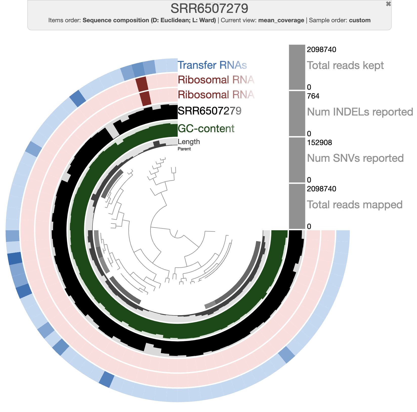
The organization of the contigs is based on their tetra-nucleotide frequency. The outer layers represent the GC content, presence of 16S and 23S rRNA as well as tRNAs. The black layers represent the mean coverage of the metagenome SRR6507279 (the metagenome associated with the sample use to generate the SAG). You can click on any part of the dendrogram to create bins. Go ahead and select all branches in the interface and go to the Bin’s tab in the setting panel. There, you will see the total size of the bin you have just created. You will also see the completion and redundancy estimation.
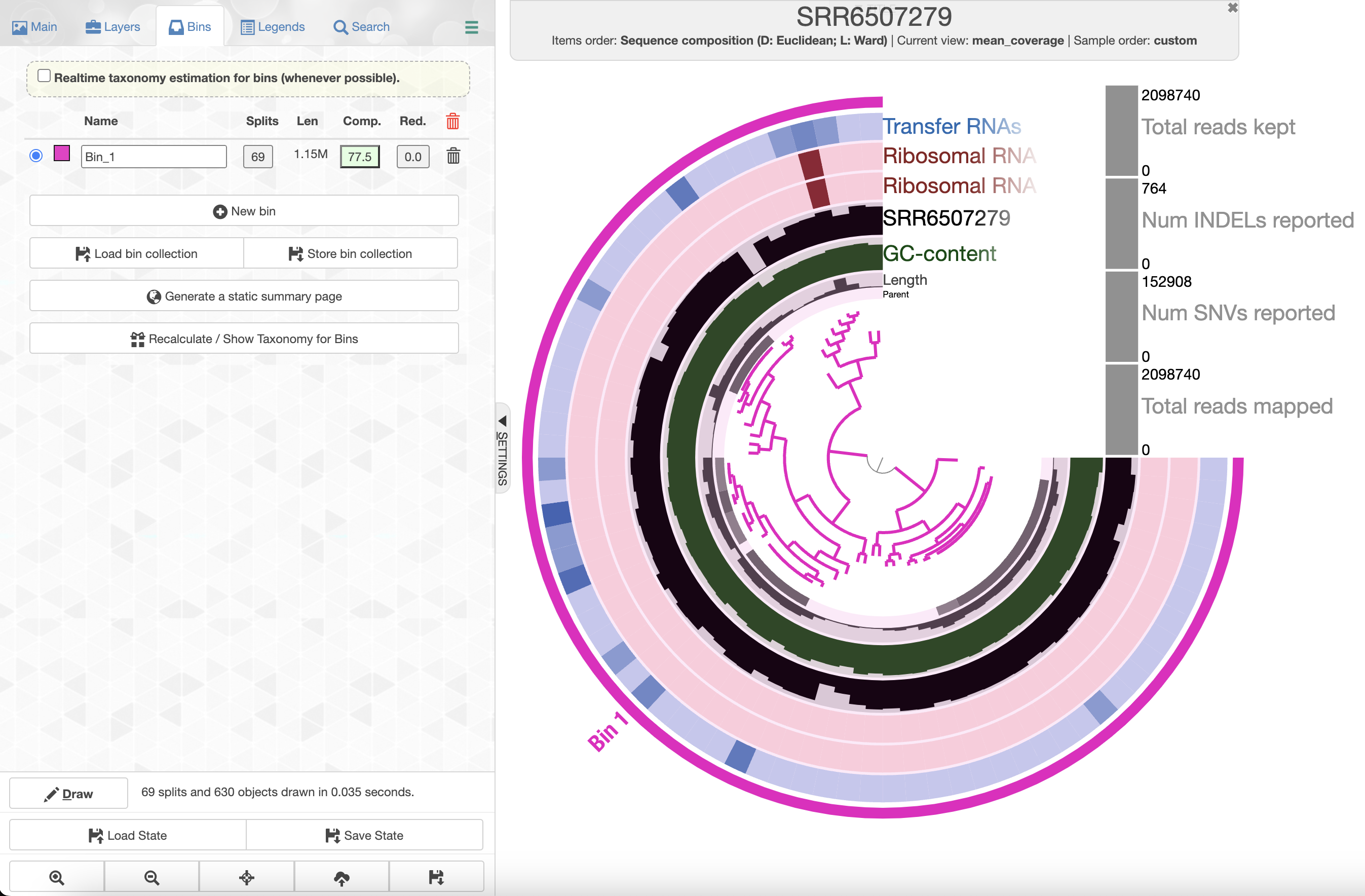
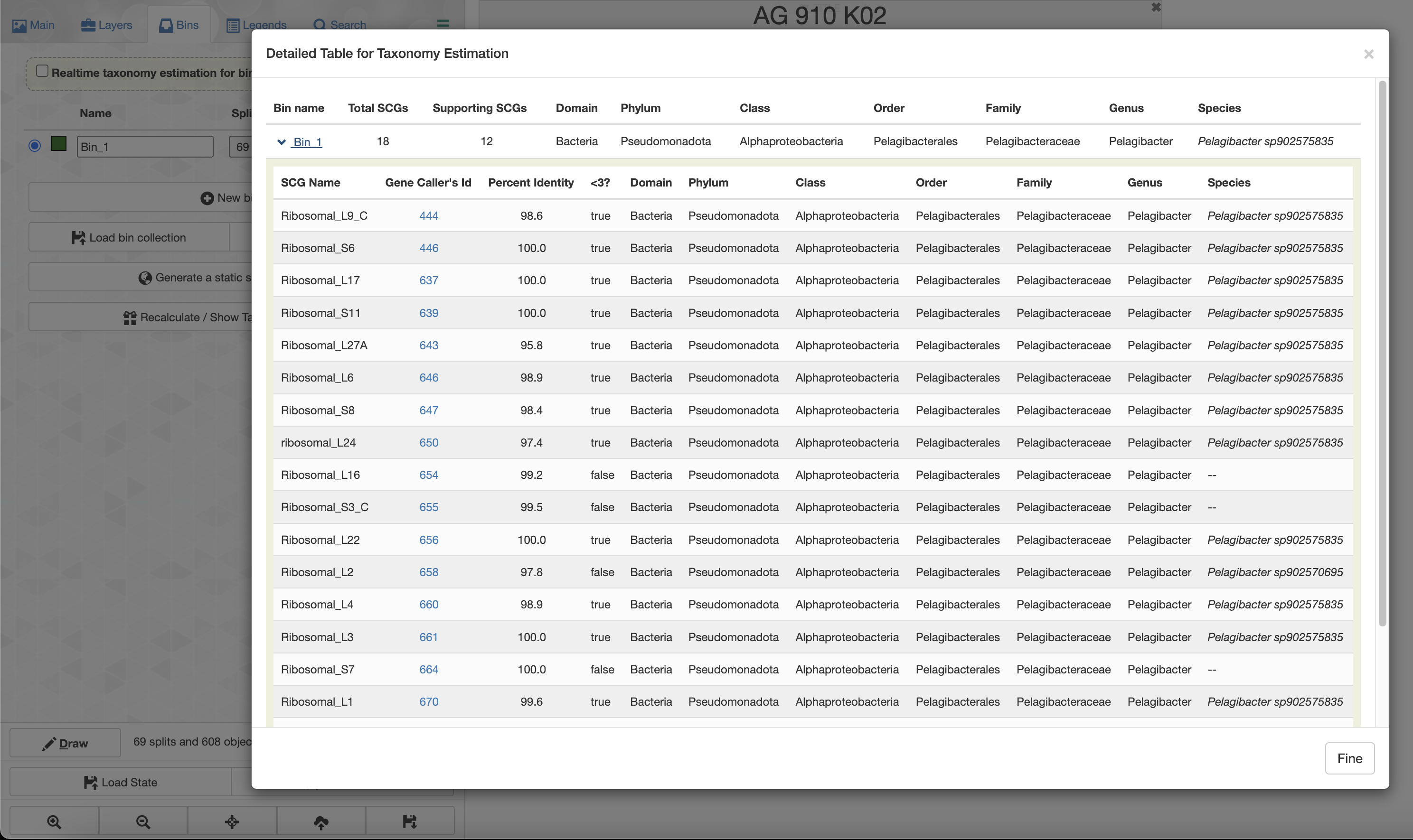
If you check the box for “Realtime taxonomy estimation for bins” you will even see the taxonomy estimation for your SAG. For more information you can click on “Recalculate/Show taxonomy for bins”, there you will be able to see the detailed taxonomic assignment for each single-copy core genes were use for taxonomy estimation.
Since we ran anvi-run-ncbi-cogs and anvi-run-kegg-kofams, we can use the Search tab in the setting panel and look for your favorite protein’s function. For instance, if you are interested in phosphate uptake by Pelagibacter you can search for the gene pst
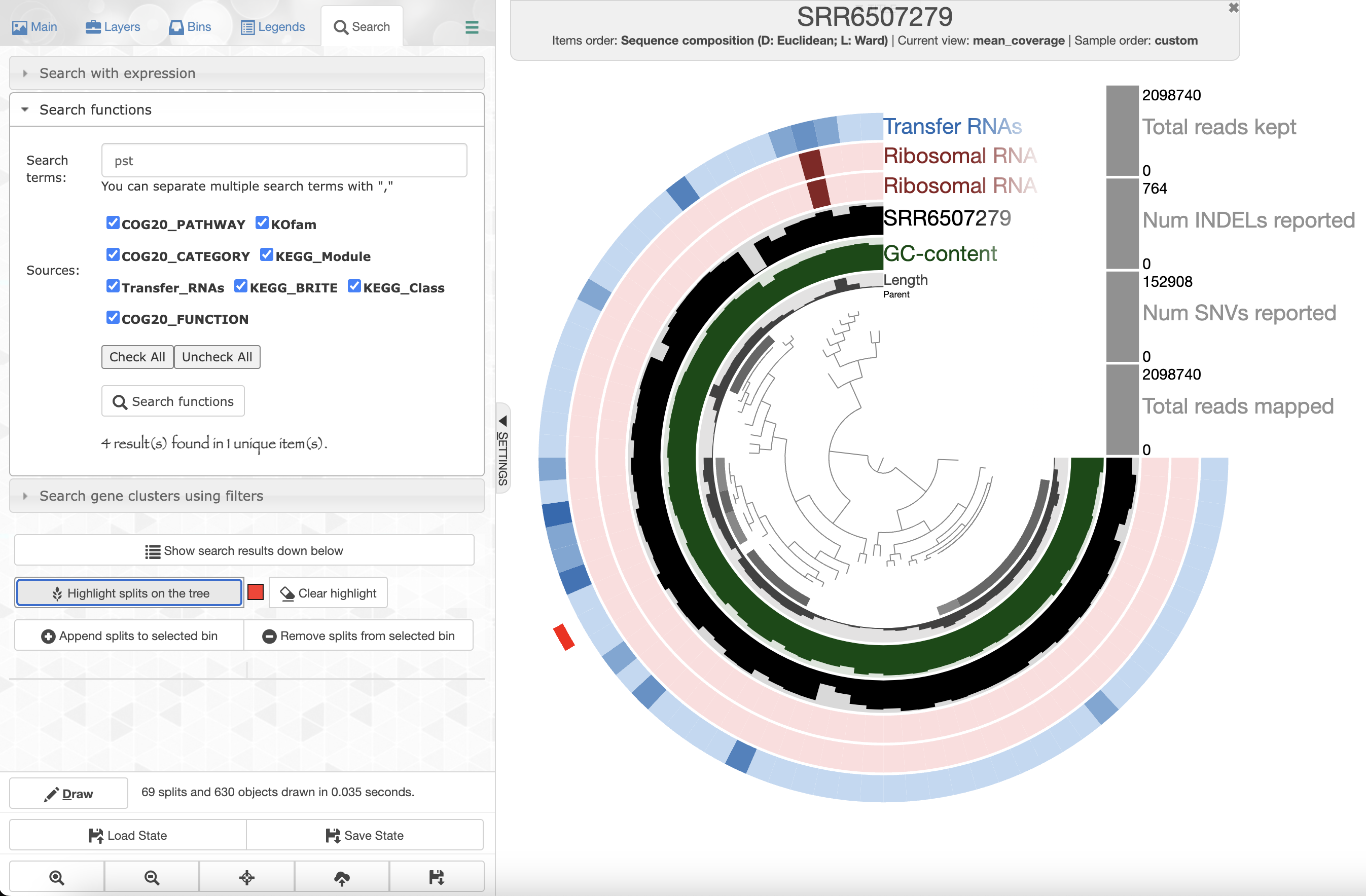
Right click on the highlighted split and select “inspect split”. It will open an inspection page as a new tab on your browser. Here you will see the read coverage along a fraction of the genome:
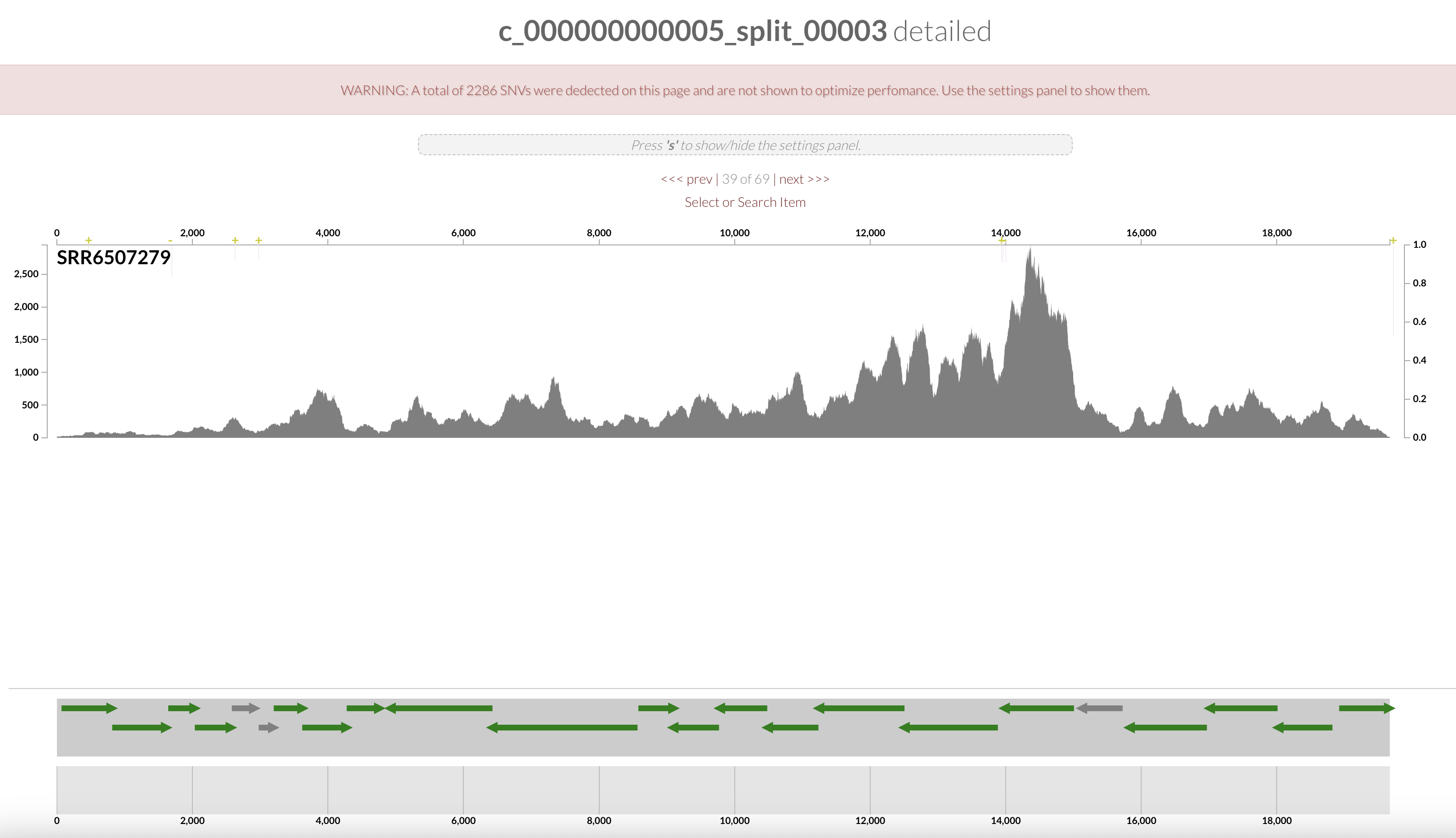
On the bottom part of the interface, you can see the ORFs and you can click on them to display information about contig’s position, length, orientation, DNA and AA sequence, quick blast options, and functional annotation when available.
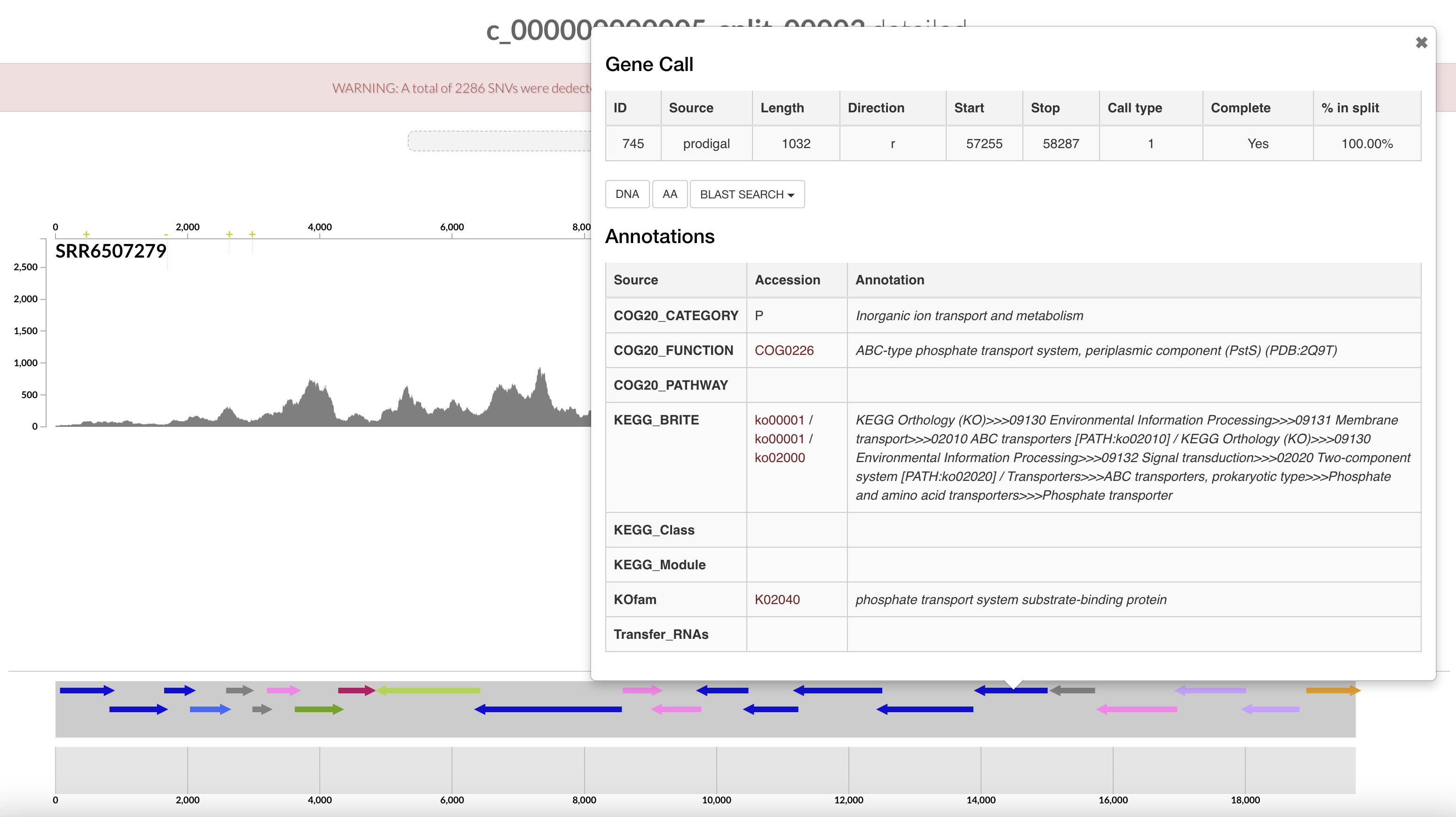
The gene’s arrows are colored based on their COG CATEGORY. If you want to change the colors, open the right side setting panel and scroll down to “Genes”. Select how you want to color the genes. You can even change individual colors.
Wonderful, you have just found the complete pstSCAB operon + PhoUB genes, which form for a high-affinity phosphate transporter.
This interactive interface allows you to investigate your genomes/assemblies manually and while it can be more intuitive than the command line, sometimes you also need excel spreadsheets. FINE. In the next sections you will learn about the command lines used to get to this point and how to comprehensively export the results of your analysis.
Create and annotate a contigs database
Let’s go back to the basics: we have a FASTA file containing our assembled SAG.
In the world of anvi’o, we put things in databases (SQLite), which are basically fancy tables. This allows for great flexibility and very easy sharing. There are different types of databases and the first one we will cover in this tutorial is the contigs-db. In it, we store the contigs’ sequences and features related to those sequences like tetra-nucleotide frequency, gene calls, DNA and amino-acid sequences, gene’s functions and taxonomy information.
Now, let’s go to the SINGLE_SAG dictionary:
cd SINGLE_SAG
To create a contigs db, we need a FASTA file of your contigs, which must have simple deflines to avoid later issues. We can use anvi-script-reformat-fasta to simplify the deflines. The flag --report-file will create a TAB-delimited file to map between the new and original deflines.
# create a directory to store the reformatted fasta file
mkdir -p FASTA

# reformat the fasta file
anvi-script-reformat-fasta DATA/AG-910-K02_contigs.fasta \
                           -o FASTA/AG-910-K02_contigs-fixed.fasta \
                           --simplify-names \
                           --report-file FASTA/AG-910-K02-reformat-report.txt
Then we can use the command anvi-gen-contigs-database to create the contigs db. When you run this command, anvi’o will identify open reading frames using Prodigal.
# create a directory for the contigs.db
mkdir -p CONTIGS

# gen the contigs.db
anvi-gen-contigs-database -f FASTA/AG-910-K02_contigs-fixed.fasta \
                          -o CONTIGS/AG-910-K02-contigs.db \
                          -n "AG_910_K02"
Annotate single-copy core genes and ribosomal RNAs
Anvi’o can use Hidden Markov Models (HMMs) of your favorite genes to find and annotate open reading frames in your contigs-db with the command anvi-run-hmms. Anvi’o comes with six sets of HMMs for ribosomal RNAs (16S, 23S, 5S, 18S, 28S, 12S), three sets of single-copy core genes (one for each domain of life). These single-copy core genes are used to compute completion and redundancy estimates.
When you run this command, a default set of HMMs will be used to annotate your database:
anvi-run-hmms --also-scan-trnas -c CONTIGS/AG-910-K02-contigs.db
If you are not interested in tRNAs, you can remove the flag --also-scan-trnas. You can always use the program anvi-scan-trnas later.
Bacteria_71 and Archaea_76 are collections that anvi’o developers curated by taking Mike Lee’s bacterial single-copy core gene collection first released in GToTree, which is an easy-to-use phylogenomics workflow.
Protista_83 is a curated collection of BUSCO by Tom Delmont.
General summary and metrics
The command anvi-display-contigs-stats takes a contigs database as input and generate an webpage-based summary with basic metrics like total DNA total length, number of contigs and genes, N50, etc. There are also some information regarding the HMM hits: number of single-copy core genes found and number of ribosomal RNAs
anvi-display-contigs-stats CONTIGS/AG-910-K02-contigs.db
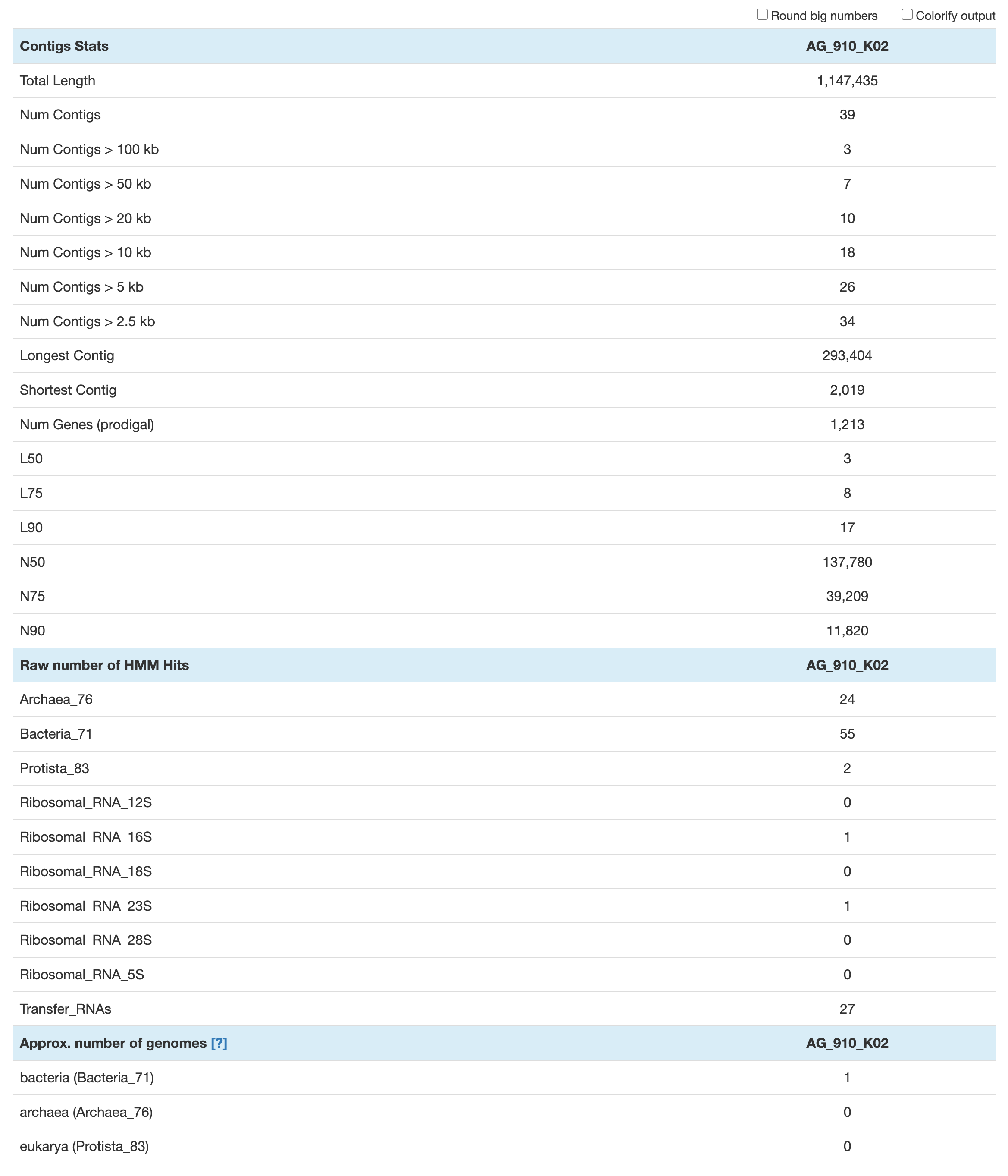
The approximate number of genomes is an estimate based on the frequency of each single-copy core gene. It is mostly useful in metagenomics, where a contigs db contains multiple microbial populations. This estimate is based on the the mode (or most frequently occurring number) of single-copy core genes. In the context of single-cell genomics, where every contigs db should represent a single population, that value should be 1 for either Archaea, Bacteria or Eukarya. If there is more than one microbial population, i.e. some contamination, that value will be over 1.
To export these metrics as a TAB-delimited file, you can use the flag --output-file, and if you don’t care about the browser interface you can also add the flag --report-as-text:
anvi-display-contigs-stats CONTIGS/AG-910-K02-contigs.db \
                           --output-file AG-910-K02-metrics.txt \
                           --report-as-text
Estimate completion and redundancy
Single-copy core genes (SCGs) are particularly useful and provide a proxy for the completeness and redundancy of a given SAG. Completeness is estimated based on the number of SCGs found in a SAG. For example, if all bacterial SCGs are found, then the genome’s completion is 100%. And if 10/100 SCGs are found in two copies, the redundancy is 10%.
Why redundancy and not contamination? The presence of multiple copies of SCGs could be indicative of a contamination in your SAG - i.e., the presence of more than one population - but microbial genomes have a bad habit of keeping a few SCGs in multiple copies. So until proven otherwise, anvi’o calls it redundancy and not contamination.
As we already have identified the SCGs with anvi-run-hmms, we can now use anvi-estimate-genome-completeness:
anvi-estimate-genome-completeness -c CONTIGS/AG-910-K02-contigs.db
You can also use the --output-file flag to generate a TAB-delimited file with the results:
anvi-estimate-genome-completeness -c CONTIGS/AG-910-K02-contigs.db \
                                  --output-file AG-910-K02-completion-redundancy.txt
| bin name | domain | confidence | % completion | % redundancy | num_splits | total length |
|---|---|---|---|---|---|---|
| AG-910-K02-contigs | BACTERIA | 0.8 | 77.46 | 0.00 | 69 | 1147435 |
Estimate SCGs taxonomy
Now that we have identified the SCGs in our SAG, anvi’o can use the Genome Taxonomy Database (GTDB) and Diamond (a fast alternative to NCBI’s BLASTp) to offer an insight into taxonomy. In a nutshell, anvi’o uses a set of SCGs (the ribosomal proteins) of the GTDB representative genome and their associated taxonomy (defined by GTDB). Each ribosomal protein gets a taxonomic assignment based on sequence similarity using Diamond.
To be able to use this function in anvi’o, you must set up SCG taxonomy once on your machine by running the command anvi-setup-scg-taxonomy.
Then we can use anvi-run-scg-taxonomy:
anvi-run-scg-taxonomy -c CONTIGS/AG-910-K02-contigs.db
This command shows you which and how many SCGs were found in your contigs db, as well as how many were taxonomically annotated. But it does not tell you what is the actual taxonomy estimation for the genome as a whole. To do that, we need to use anvi-estimate-scg-taxonomy to report the consensus taxonomic estimation for all Ribosomal protein in this SAG (using the --output-file flag to store the result):
anvi-estimate-scg-taxonomy -c CONTIGS/AG-910-K02-contigs.db \
                           --output-file AG-910-K02-taxonomy.txt
| bin_name | total_scgs | supporting_scgs | t_domain | t_phylum | t_class | t_order | t_family | t_genus | t_species |
|---|---|---|---|---|---|---|---|---|---|
| AG_910_K02 | 18 | 12 | Bacteria | Proteobacteria | Alphaproteobacteria | Pelagibacterales | Pelagibacteraceae | Pelagibacter | Pelagibacter sp902575835 |
The total number of SCGs represents the number of SCGs found in this SAG that were usable for taxonomy estimation, and the number of supporting SCGs represents the number of SCGs matching the consensus taxonomy.
Only 12 out of 18 SCGs match the consensus taxonomy. We can inspect each SCGs taxonomic affiliation by using the --debug flag:
$ anvi-estimate-scg-taxonomy -c CONTIGS/AG-910-K02-contigs.db --debug
Contigs DB ...................................: CONTIGS/AG-910-K02-contigs.db
Metagenome mode ..............................: False

* A total of 18 single-copy core genes with taxonomic affiliations were
  successfully initialized from the contigs database 🎉 Following shows the
  frequency of these SCGs: Ribosomal_S3_C (1), Ribosomal_S6 (1), Ribosomal_S7
  (1), Ribosomal_S8 (1), Ribosomal_S11 (1), Ribosomal_S20p (1), Ribosomal_L1
  (1), Ribosomal_L2 (1), Ribosomal_L3 (1), Ribosomal_L4 (1), Ribosomal_L6 (1),
  Ribosomal_L9_C (1), Ribosomal_L16 (1), Ribosomal_L17 (1), Ribosomal_L20 (1),
  Ribosomal_L22 (1), ribosomal_L24 (1), Ribosomal_L27A (1), Ribosomal_S2 (0),
  Ribosomal_S9 (0), Ribosomal_L13 (0), Ribosomal_L21p (0).

Hits for AG_910_K02
===============================================
+----------------+--------+----------+----------------------------------------------------------------------------------------------------------------------------------+
| SCG            | gene   | pct id   | taxonomy                                                                                                                         |
+================+========+==========+==================================================================================================================================+
| Ribosomal_L27A | 643    | 95.8     | Bacteria / Pseudomonadota / Alphaproteobacteria / Pelagibacterales / Pelagibacteraceae / Pelagibacter / Pelagibacter sp902575835 |
+----------------+--------+----------+----------------------------------------------------------------------------------------------------------------------------------+
| Ribosomal_S20p | 964    | 100.0    | Bacteria / Pseudomonadota / Alphaproteobacteria / Pelagibacterales / Pelagibacteraceae / Pelagibacter /                          |
+----------------+--------+----------+----------------------------------------------------------------------------------------------------------------------------------+
| Ribosomal_L20  | 773    | 100.0    | Bacteria / Pseudomonadota / Alphaproteobacteria / Pelagibacterales / Pelagibacteraceae / Pelagibacter /                          |
+----------------+--------+----------+----------------------------------------------------------------------------------------------------------------------------------+
| Ribosomal_L6   | 646    | 98.9     | Bacteria / Pseudomonadota / Alphaproteobacteria / Pelagibacterales / Pelagibacteraceae / Pelagibacter / Pelagibacter sp902575835 |
+----------------+--------+----------+----------------------------------------------------------------------------------------------------------------------------------+
| Ribosomal_S8   | 647    | 98.4     | Bacteria / Pseudomonadota / Alphaproteobacteria / Pelagibacterales / Pelagibacteraceae / Pelagibacter / Pelagibacter sp902575835 |
+----------------+--------+----------+----------------------------------------------------------------------------------------------------------------------------------+
| ribosomal_L24  | 650    | 97.4     | Bacteria / Pseudomonadota / Alphaproteobacteria / Pelagibacterales / Pelagibacteraceae / Pelagibacter / Pelagibacter sp902575835 |
+----------------+--------+----------+----------------------------------------------------------------------------------------------------------------------------------+
| Ribosomal_L16  | 654    | 99.2     | Bacteria / Pseudomonadota / Alphaproteobacteria / Pelagibacterales / Pelagibacteraceae / Pelagibacter /                          |
+----------------+--------+----------+----------------------------------------------------------------------------------------------------------------------------------+
| Ribosomal_S3_C | 655    | 99.5     | Bacteria / Pseudomonadota / Alphaproteobacteria / Pelagibacterales / Pelagibacteraceae / Pelagibacter /                          |
+----------------+--------+----------+----------------------------------------------------------------------------------------------------------------------------------+
| Ribosomal_L22  | 656    | 100.0    | Bacteria / Pseudomonadota / Alphaproteobacteria / Pelagibacterales / Pelagibacteraceae / Pelagibacter / Pelagibacter sp902575835 |
+----------------+--------+----------+----------------------------------------------------------------------------------------------------------------------------------+
| Ribosomal_L2   | 658    | 97.8     | Bacteria / Pseudomonadota / Alphaproteobacteria / Pelagibacterales / Pelagibacteraceae / Pelagibacter / Pelagibacter sp902570695 |
+----------------+--------+----------+----------------------------------------------------------------------------------------------------------------------------------+
| Ribosomal_L4   | 660    | 98.9     | Bacteria / Pseudomonadota / Alphaproteobacteria / Pelagibacterales / Pelagibacteraceae / Pelagibacter / Pelagibacter sp902575835 |
+----------------+--------+----------+----------------------------------------------------------------------------------------------------------------------------------+
| Ribosomal_L3   | 661    | 100.0    | Bacteria / Pseudomonadota / Alphaproteobacteria / Pelagibacterales / Pelagibacteraceae / Pelagibacter / Pelagibacter sp902575835 |
+----------------+--------+----------+----------------------------------------------------------------------------------------------------------------------------------+
| Ribosomal_S7   | 664    | 100.0    | Bacteria / Pseudomonadota / Alphaproteobacteria / Pelagibacterales / Pelagibacteraceae / Pelagibacter /                          |
+----------------+--------+----------+----------------------------------------------------------------------------------------------------------------------------------+
| Ribosomal_L1   | 670    | 99.6     | Bacteria / Pseudomonadota / Alphaproteobacteria / Pelagibacterales / Pelagibacteraceae / Pelagibacter / Pelagibacter sp902575835 |
+----------------+--------+----------+----------------------------------------------------------------------------------------------------------------------------------+
| Ribosomal_L9_C | 444    | 98.6     | Bacteria / Pseudomonadota / Alphaproteobacteria / Pelagibacterales / Pelagibacteraceae / Pelagibacter / Pelagibacter sp902575835 |
+----------------+--------+----------+----------------------------------------------------------------------------------------------------------------------------------+
| Ribosomal_L17  | 637    | 100.0    | Bacteria / Pseudomonadota / Alphaproteobacteria / Pelagibacterales / Pelagibacteraceae / Pelagibacter / Pelagibacter sp902575835 |
+----------------+--------+----------+----------------------------------------------------------------------------------------------------------------------------------+
| Ribosomal_S6   | 446    | 100.0    | Bacteria / Pseudomonadota / Alphaproteobacteria / Pelagibacterales / Pelagibacteraceae / Pelagibacter / Pelagibacter sp902575835 |
+----------------+--------+----------+----------------------------------------------------------------------------------------------------------------------------------+
| Ribosomal_S11  | 639    | 100.0    | Bacteria / Pseudomonadota / Alphaproteobacteria / Pelagibacterales / Pelagibacteraceae / Pelagibacter / Pelagibacter sp902575835 |
+----------------+--------+----------+----------------------------------------------------------------------------------------------------------------------------------+
| CONSENSUS      | --     | --       | Bacteria / Pseudomonadota / Alphaproteobacteria / Pelagibacterales / Pelagibacteraceae / Pelagibacter / Pelagibacter sp902575835 |
+----------------+--------+----------+----------------------------------------------------------------------------------------------------------------------------------+

Estimated taxonomy for "AG_910_K02"
===============================================
+------------+--------------+-------------------+----------------------------------------------------------------------------------------------------------------------------------+
|            |   total_scgs |   supporting_scgs | taxonomy                                                                                                                         |
+============+==============+===================+==================================================================================================================================+
| AG_910_K02 |           18 |                12 | Bacteria / Pseudomonadota / Alphaproteobacteria / Pelagibacterales / Pelagibacteraceae / Pelagibacter / Pelagibacter sp902575835 |
+------------+--------------+-------------------+----------------------------------------------------------------------------------------------------------------------------------+
Now we can see that the 6 SCGs that were not matching the consensus Pelagibacter sp902575835 were matching to the genus Pelagibacter or to Pelagibacter sp902570695.
Anvi’o’s strategy for estimating taxonomy is limited to Archaea and Bacteria since it uses GTDB, and anvi’o will not estimate taxonomy for a SAG with low completion based on the number of SCGs. It is not a perfect way to estimate taxonomy but it is very fast.
Functional annotations
There are multiple databases out there that we can use to investigate gene functions. Each of these databases fills a specific need and none of them are perfect. A database like NCBI’s clusters of orthologous groups (COG) will give general annotations, while the KEGG database offers more precise annotations with metabolism-related genes, and others like Pfam focus on protein families. Anvi’o can use these three databases to annotate open reading frames, and you can also import any functional annotations generated with a third party software.
You can import your own functional annotations into anvi’o. Let’s imagine you really want to look for carbohydrate-active enzymes using the CAZy database. Well, you can export the gene sequences (DNA or amino acid) using anvi-get-sequences-for-gene-calls, annotate your genes with CAZy (or your favorite tool and/or database), and import the results back into the contigs db with anvi-import-functions.
For this analysis, we will use COG and KEGG annotations. To be able to run these annotations, we first need to download and set up the COG and KEGG databases locally using anvi-setup-ncbi-cogs and anvi-setup-kegg-kofams. Like we did for the SCG taxonomy data, we only need to run these commands once, after which the data will be stored on our machines.
If you have these two databases set up, you can annotate your contigs db with anvi-run-ncbi-cogs and anvi-run-kegg-kofams:
anvi-run-ncbi-cogs -c CONTIGS/AG-910-K02-contigs.db -T 4
anvi-run-kegg-kofams -c CONTIGS/AG-910-K02-contigs.db -T 4
To export the functional annotations from the database as TAB-delimited files, you can use anvi-export-functions. For this command you will have to specify which annotation source you want to use. If you are unsure what functional annotations were carried out on your contigs db, you can use the flag --list-annotation-sources:
anvi-export-functions -c CONTIGS/AG-910-K02-contigs.db \
                      --list-annotation-sources


FUNCTIONAL ANNOTATION SOURCES FOUND
===============================================
* COG20_PATHWAY
* COG20_FUNCTION
* KEGG_Module
* KEGG_Class
* KOfam
* COG20_CATEGORY
Then we can export the COG annotations:
anvi-export-functions -c CONTIGS/AG-910-K02-contigs.db \
                      --annotation-sources COG20_FUNCTION \
                      --output-file AG-910-K02-COG20_FUNCTION.txt
And the output file should be a table that looks like this:
| gene_callers_id | source | accession | function | e_value |
|---|---|---|---|---|
| 0 | COG20_FUNCTION | COG4091 | Predicted homoserine dehydrogenase, contains C-terminal SAF domain (PDB:3UPL) | 9.9e-179 |
| 1 | COG20_FUNCTION | COG4392 | Branched-chain amino acid transport protein (AzlD2) | 1.2e-21 |
| 2 | COG20_FUNCTION | COG1296 | Predicted branched-chain amino acid permease (azaleucine resistance) (AzlC) | 2.4e-59 |
| 3 | COG20_FUNCTION | COG2105 | Predicted gamma-glutamylamine cyclotransferase YtfP, GGCT/AIG2-like family (YtfP) (PDB:1V30) (PUBMED:16754964;20110353) | 6.5e-12 |
| 4 | COG20_FUNCTION | COG1058 | ADP-ribose pyrophosphatase domain of DNA damage- and competence-inducible protein CinA (CinA) (PDB:4CT9) (PUBMED:25313401) | 5.9e-67 |
| -- | -- | -- | -- | -- |
| 1209 | COG20_FUNCTION | COG0396 | Fe-S cluster assembly ATPase SufC (SufC) (PDB:2D3W) | 2e-91 |
| 1210 | COG20_FUNCTION | COG0719 | Fe-S cluster assembly scaffold protein SufB (SufB) (PDB:1VH4) | 2.2e-204 |
| 1211 | COG20_FUNCTION | COG3808 | Na+ or H+-translocating membrane pyrophosphatase (OVP1) (PDB:4A01) (PUBMED:11342551) | 7.7e-281 |
Remember the pstSCAB + PhoU operon for inorganic phosphate transport that we identified in the interactive interface? We can search for them in the output generated above:
$ grep -e "Pst" -e "PhoU" AG-910-K02-COG20_FUNCTION.txt
741	COG20_FUNCTION	COG0704	Phosphate uptake regulator PhoU (PhoU) (PDB:1T8B)	7.09e-69
742	COG20_FUNCTION	COG1117	ABC-type phosphate transport system, ATPase component (PstB)	8.3e-145
743	COG20_FUNCTION	COG0581	ABC-type phosphate transport system, permease component (PstA)	6.15e-175
744	COG20_FUNCTION	COG0573	ABC-type phosphate transport system, permease component (PstC)	3.04e-184
745	COG20_FUNCTION	COG0226	ABC-type phosphate transport system, periplasmic component (PstS) (PDB:2Q9T)	5.64e-144
You can use anvi-export-gene-calls to get the gene’s DNA/amino-acid sequence.
Estimate KEGG module completion
What makes the KEGG database unique is its ability to contextualize annotations into functional modules and pathways. We can use the program anvi-estimate-metabolism to estimate the completion of KEGG modules for our SAG:
anvi-estimate-metabolism -c CONTIGS/AG-910-K02-contigs.db
It will generate a TAB-delimited file where each row represents a KEGG module, its name, the associated KOs, the completeness of the module in the SAG, and more:
unique_id	genome_name	kegg_module	module_name	module_class	module_category	module_subcategory	module_definition	module_completeness	module_is_complete	kofam_hits_in_module	gene_caller_ids_in_module	warnings
0	AG_910_K02	M00001	Glycolysis (Embden-Meyerhof pathway), glucose => pyruvate	Pathway modules	Carbohydrate metabolism	Central carbohydrate metabolism	"(K00844,K12407,K00845,K00886,K08074,K00918) (K01810,K06859,K13810,K15916) (K00850,K16370,K21071,K00918) (K01623,K01624,K11645,K16305,K16306) K01803 ((K00134,K00150) K00927,K11389) (K01834,K15633,K15634,K15635) K01689 (K00873,K12406)"	0.3	False	K00134,K00927,K01623	1045,1046,1047	None
1	AG_910_K02	M00002	Glycolysis, core module involving three-carbon compounds	Pathway modules	Carbohydrate metabolism	Central carbohydrate metabolism	"K01803 ((K00134,K00150) K00927,K11389) (K01834,K15633,K15634,K15635) K01689 (K00873,K12406)"	0.3333333333333333	False	K00134,K00927	1045,1046	None
2	AG_910_K02	M00003	Gluconeogenesis, oxaloacetate => fructose-6P	Pathway modules	Carbohydrate metabolism	Central carbohydrate metabolism	"(K01596,K01610) K01689 (K01834,K15633,K15634,K15635) K00927 (K00134,K00150) K01803 ((K01623,K01624,K11645) (K03841,K02446,K11532,K01086,K04041),K01622)"	0.375	False	K00134,K00927,K01623	1045,1046,1047	None
3	AG_910_K02	M00307	Pyruvate oxidation, pyruvate => acetyl-CoA	Pathway modules	Carbohydrate metabolism	Central carbohydrate metabolism	"((K00163,K00161+K00162)+K00627+K00382-K13997),K00169+K00170+K00171+(K00172,K00189),K03737"	1.0	True	K00163,K00163,K00382,K00627	761,230,467,762	None
4	AG_910_K02	M00009	Citrate cycle (TCA cycle, Krebs cycle)	Pathway modules	Carbohydrate metabolism	Central carbohydrate metabolism	"(K01647,K05942) (K01681,K01682) (K00031,K00030) (K00164+K00658+K00382,K00174+K00175-K00177-K00176) (K01902+K01903,K01899+K01900,K18118) (K00234+K00235+K00236+K00237,K00239+K00240+K00241-(K00242,K18859,K18860),K00244+K00245+K00246-K00247) (K01676,K01679,K01677+K01678) (K00026,K00025,K00024,K00116)"	0.875	True	K00024,K00031,K00164,K00239,K00240,K00241,K00242,K00382,K00658,K01679,K01681,K01902,K01903	472,390,469,475,474,477,476,467,468,369,156,470,471	None
5	AG_910_K02	M00010	Citrate cycle, first carbon oxidation, oxaloacetate => 2-oxoglutarate	Pathway modules	Carbohydrate metabolism	Central carbohydrate metabolism	"(K01647,K05942) (K01681,K01682) (K00031,K00030)"	0.6666666666666666	False	K00031,K01681	390,156	None
6	AG_910_K02	M00011	Citrate cycle, second carbon oxidation, 2-oxoglutarate => oxaloacetate	Pathway modules	Carbohydrate metabolism	Central carbohydrate metabolism	"(K00164+K00658+K00382,K00174+K00175-K00177-K00176) (K01902+K01903,K01899+K01900,K18118) (K00234+K00235+K00236+K00237,K00239+K00240+K00241-(K00242,K18859,K18860),K00244+K00245+K00246-K00247) (K01676,K01679,K01677+K01678) (K00026,K00025,K00024,K00116)"	1.0	True	K00024,K00164,K00239,K00240,K00241,K00242,K00382,K00658,K01679,K01902,K01903	472,469,475,474,477,476,467,468,369,470,471	None
7	AG_910_K02	M00004	Pentose phosphate pathway (Pentose phosphate cycle)	Pathway modules	Carbohydrate metabolism	Central carbohydrate metabolism	"(K13937,((K00036,K19243) (K01057,K07404))) K00033 K01783 (K01807,K01808) K00615 K00616 (K01810,K06859,K13810,K15916)"	0.5714285714285714	False	K00615,K00616,K01783,K01808	1044,1053,550,601	None
8	AG_910_K02	M00007	Pentose phosphate pathway, non-oxidative phase, fructose 6P => ribose 5P	Pathway modules	Carbohydrate metabolism	Central carbohydrate metabolism	"K00615 (K00616,K13810) K01783 (K01807,K01808)"	1.0	True	K00615,K00616,K01783,K01808	1044,1053,550,601	None
By default, anvi’o labels a module as ‘present’ if its completeness is > 0.75. We are using SAGs, which are inherently incomplete, so be very critical about this completeness threshold (which you can change using the flag --module-completion-threshold).
Generate a profile database to use anvi-interactive
Now that a completely annotated contigs-db you maybe wonder how to visualize it just like in the first part of this tutorial? If you look at the help page for anvi-interactive you would see that it requires a profile-db.
profile-db are used to store read-recruitment results, which we don’t have at the moment. We can use anvi-profile with the flag –blank to generate an empty profile-db.
anvi-profile --blank -c CONTIGS/AG-910-K02-contigs.db -o PROFILE -S AG_910_K02
Now you are ready to start and interactive interface:
anvi-interactive -c CONTIGS/AG-910-K02-contigs.db -p PROFILE/PROFILE.db
Now we went through all the basics of analyzing a single SAG in anvi’o. However, in real life we often have many SAGs that we want to analyze all at once. Now we will learn how to do this.
Working with multiple SAGs
Let’s step up our game and repeat the above analyses for the 228 SAGs in the AG-910 sample!
You can change your current working directory to MULTIPLE_SAGs:
cd ../MULTIPLE_SAGs
And this is what you should see in it:
$ ls
ADDITIONAL_DATA DATA
With 226 contigs databases in the DATA directory.
All of the contigs databases are already provided and were annotated in the same way as shown above with AG_910_K02. The reason why we already did all of this is pretty simple: it takes a lot of time and/or computer resource. But now that you know how to generate and annotate one contigs db, you could do this for many databases at a time - for instance, by using bash loops. But loops would not be the most effective way to do it. If you have access to a more powerful machine like a computing cluster, you can check out the anvi’o workflows. Basically, you can use anvi-run-workflow to automatically run all the steps to generate a set of contigs databases, a full metagenomics workflow (including assembly, short-read mapping, anvi’o profiles and more), pangenomics, phylogenomics and more. It uses snakemake, a very powerful workflow management system.
General metrics
We’ve previously used anvi-display-contigs-stats to export some information about a single SAG like its length, number of contigs, number of single-copy core genes and more. If you look at the help menu of that command, you will see that it can accept as many contigs databases as you wish.
Let’s run it using all of the contigs databases available in the datapack:
anvi-display-contigs-stats --output-file stats.txt DATA/*contigs.db
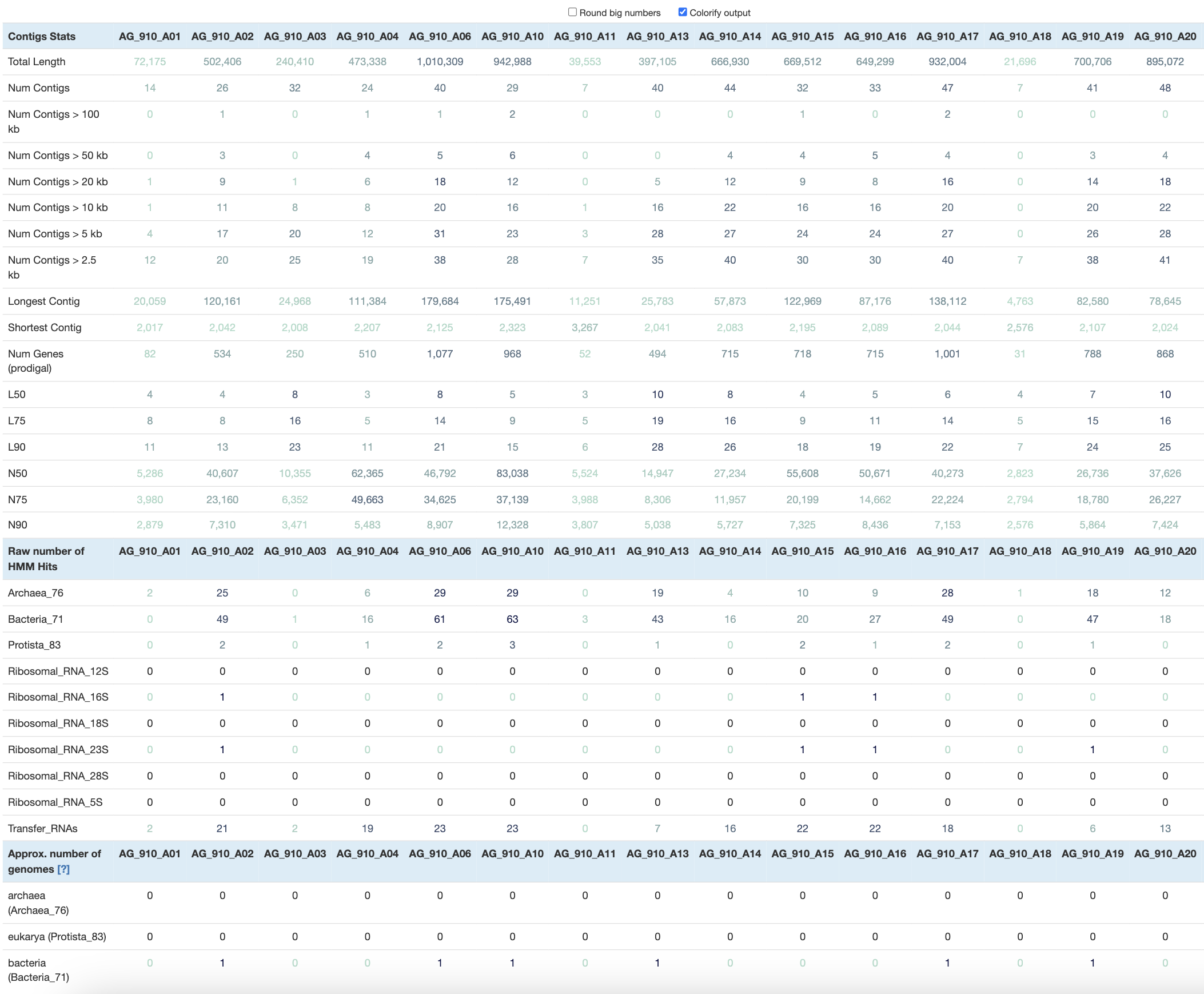
At this point, the interactive interface includes a table with over 200 columns, which is a bit overwhelming. To make more sense of the numbers, you can click on Colorify output to visually appreciate high and low values in each row.
With the --output-file flag, you will save that table as a TAB-delimited file and import it in your favorite table-eating software like R, Python and others (we also use Excel sometimes). You will be able to compute the total size distribution of all the SAGs, calculate the average number of contigs, and select SAGs based on your favorite metric!
Completeness and redundancy
While anvi-display-contigs-stats was very happy to take as many contigs databases as possible, it is not the case with other programs in anvi’o.
Here is what you can find in the help manual of anvi-estimate-genome-completeness:
MANDATORY INPUT OPTION #2
  Or you can initiate this with an external genomes file.

  -e FILE_PATH, --external-genomes FILE_PATH
                        A two-column TAB-delimited flat text file that lists
                        anvi'o contigs databases. The first item in the header
                        line should read 'name', and the second should read
                        'contigs_db_path'. Each line in the file should
                        describe a single entry, where the first column is the
                        name of the genome (or MAG), and the second column is
                        the anvi'o contigs database generated for this genome.
                        (default: None)
You can use an external-genomes file containing the names and paths to your contigs databases. While you can manually generate that file, there is a very convenient command in anvi’o that will do it for you: anvi-script-gen-genomes-file. Let’s use it:
anvi-script-gen-genomes-file --input-dir DATA \
                             -o external-genomes.txt
And here is how the file should look like:
$ head -n 10 external-genomes.txt
name	contigs_db_path
AG_910_A01	/path/to/MULTIPLE_SAGs/DATA/AG_910_A01-contigs.db
AG_910_A02	/path/to/MULTIPLE_SAGs/DATA/AG_910_A02-contigs.db
AG_910_A03	/path/to/MULTIPLE_SAGs/DATA/AG_910_A03-contigs.db
AG_910_A04	/path/to/MULTIPLE_SAGs/DATA/AG_910_A04-contigs.db
AG_910_A06	/path/to/MULTIPLE_SAGs/DATA/AG_910_A06-contigs.db
AG_910_A10	/path/to/MULTIPLE_SAGs/DATA/AG_910_A10-contigs.db
AG_910_A11	/path/to/MULTIPLE_SAGs/DATA/AG_910_A11-contigs.db
AG_910_A13	/path/to/MULTIPLE_SAGs/DATA/AG_910_A13-contigs.db
AG_910_A14	/path/to/MULTIPLE_SAGs/DATA/AG_910_A14-contigs.db
We can now use anvi-estimate-genome-completeness with the external-genomes file instead of a single contigs db:
anvi-estimate-genome-completeness -e external-genomes.txt \
                                  --output-file completion-redundancy.txt
Use bash to get the most complete SAGs
Let’s imagine that you are interested in the top 5 most complete SAGs. You can use the bash command sort and head to quickly create and store a list of these SAGs’ names in a file.
For sort, the n flag stands for numerical, the r flag is for reverse sorting (descending order), and the k flag is for specifying which column you want to do the sorting on. The completeness estimate is in the 4th column in completion-redundancy.txt, so we use k4.
Then, we can use head to select only the first 5 lines.
$ sort -nrk4 completion-redundancy.txt | head -n 5

AG_910_D13	BACTERIA	1.0	94.37	0.00	73	1117975
AG_910_M21	BACTERIA	1.0	91.55	0.00	48	910570
AG_910_L17	BACTERIA	0.9	90.14	0.00	58	1089091
AG_910_C02	BACTERIA	0.9	90.14	0.00	55	936322
AG_910_B21	BACTERIA	0.9	90.14	2.82	114	1930694
If you want to store the list of SAG names in a file, you can use cut to select only the first column:
sort -nrk4 completion-redundancy.txt | head -n 5 | cut -f 1 > five_most_complete_SAGs.txt
Taxonomy estimation
Our next step is to investigate the taxonomy of all the SAGs. We need to use anvi-estimate-scg-taxonomy, which unfortunately does not use an external genomes file. No one is perfect, but you can find and shame an anvi’o developer by using the discord server, or anvi’o github for a feature request like this.
If you really want the taxonomy of all your SAGs (and it is your right), there is a way with the power of bash!
First of all, you want to loop through every SAG and run anvi-estimate-scg-taxonomy.
You can use the while loop with the external genomes file. Basically, you create two variables that correspond to the columns of your file. The if line is there to skip the header of the external genomes file.
# create a directory to store all the outputs
mkdir -p TAXONOMY

# going through each SAGs at a time
# it will take a few min
while read name path
do
  if [ "$name" == "name" ]; then continue; fi
  anvi-estimate-scg-taxonomy -c $path -o TAXONOMY/$name.txt
done < external-genomes.txt
Once all you have all the output, you can merge them with a similar while loop.
# take the header line and create the general output
head -n 1 TAXONOMY/AG_910_A01.txt > taxonomy.txt

# append each SAG's output to the final file
while read name path; do
  if [ "$name" == "name" ]; then continue; fi
  sed 1d TAXONOMY/$name.txt >> taxonomy.txt
done < external-genomes.txt
sed 1d is used to remove the first line (table header).
Now you have the final taxonomy output for all your SAGs! Are you interested in Pelagibacter? You can search for all the SAGs with a Pelagibacter assignment:
$ grep Pelagibacter taxonomy.txt
AG_910_A06	19	9	Bacteria	Proteobacteria	Alphaproteobacteria	Pelagibacterales	Pelagibacteraceae	Pelagibacter	Pelagibacter sp902567045
AG_910_A11	1	1	Bacteria	Proteobacteria	Alphaproteobacteria	Pelagibacterales	Pelagibacteraceae	Pelagibacter	Pelagibacter sp902612325
AG_910_A14	4	4	Bacteria	Proteobacteria	Alphaproteobacteria	Pelagibacterales	AG-422-B15	AG-422-B15	None
AG_910_A15	6	4	Bacteria	Proteobacteria	Alphaproteobacteria	Pelagibacterales	Pelagibacteraceae	Pelagibacter	Pelagibacter sp902573345
AG_910_A17	17	17	Bacteria	Proteobacteria	Alphaproteobacteria	Pelagibacterales	Pelagibacteraceae	Pelagibacter	None
---
Metabolic pathway completeness
The program anvi-estimate-metabolism allows you to predict the metabolic capabilities of an organism. It is based on the KEGG’s module, but you can also use user-defined pathways. We will cover both in the next sections.
Estimate KEGG module completion
This section of the tutorial is heavily inspired by this comprehensive tutorial about metabolic reconstruction in anvi’o
anvi-estimate-metabolism can also use an external-genomes as an input parameter. This program can also output multiple type of tables and since we have multiple SAGs, we could be interested in a matrix-format table where SAGs are columns and rows are KEGG’s module. The following command line also include the flag --include-metadata which will add a column with metadata for each module, like module name and category:
anvi-estimate-metabolism -e external-genomes-50.txt \
                         -O SAG \
                         --matrix-format \
                         --include-metadata
That command generated 6 output files, including matrices of the stepwise and pathwise completeness and presence (which is a binary table based on your completion threshold); as well as a matrix of module’s individual steps and the number of copies of each KOfam annotation.
Let’s visualize the matrix of the pathwise completion using anvi-interactive in manual mode:
anvi-interactive -d SAG-module_pathwise_completeness-MATRIX.txt \
                 -p modules_heatmap.db \
                 --manual \
                 --title "Metabolism heatmap"
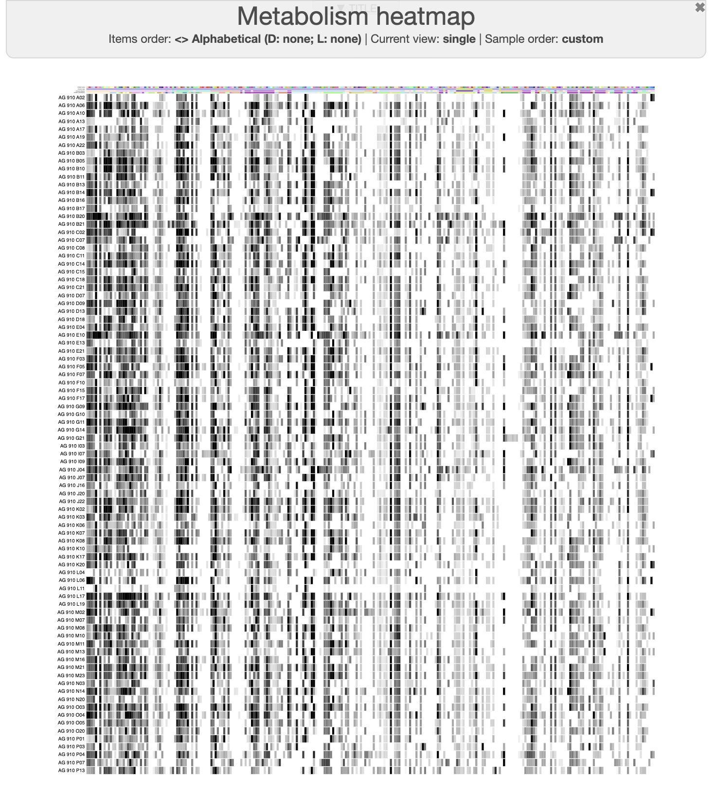
To reproduce this figure, you will need to set the ‘Drawing type’ to phylogram, increase the width to ~15,000, and for each SAG layer you need to change the type to “intensity”.
To organize the data in a nicer way, we can cluster both the SAGs and the module based on the matrix value. First we can cluster the pathway so that metabolism with similar SAG distribution come together on the interactive interface. First, we need to remove the metadata columns because anvi-matrix-to-newick expects only numbers in the input:
cut -f1,6- SAG-module_pathwise_completeness-MATRIX.txt > SAG-module_pathwise_completeness-MATRIX-NO-METADATA.txt
anvi-matrix-to-newick SAG-module_pathwise_completeness-MATRIX-NO-METADATA.txt -o module_organization.newick
Now we can transpose the table and do the same for the SAG organisation:
anvi-script-transpose-matrix SAG-module_pathwise_completeness-MATRIX-NO-METADATA.txt \
                             -o SAG-module_pathwise_completeness-MATRIX-NO-METADATA-TRANSPOSE.txt
anvi-matrix-to-newick SAG-module_pathwise_completeness-MATRIX-NO-METADATA-TRANSPOSE.txt -o SAG_organization.newick
We have now two dendrogram fro each side of our heatmap and we can integrate them to the interactive interface. We can import the module_organisation.newick using anvi-import-items-order:
anvi-import-items-order -i module_organization.newick \
                        -p modules_heatmap.db \
                        --name module_organization
In the interface, the SAG are present in the “layer” section. So we need to use a different command to import SAG_organization.newick: anvi-import-misc-data:
# format the input data a bit
TREE=$(cat SAG_organization.newick)
echo -e "item_name\tdata_type\tdata_value\nSAG_organization\tnewick\t$TREE" > layer_order.txt
# import into the database
anvi-import-misc-data -p modules_heatmap.db \
                      -t layer_orders \
                      layer_order.txt
But why stop here? Let’s add the SAG’s taxonomy:
anvi-import-misc-data -p modules_heatmap.db \
                      -t layers \
                      taxonomy.txt
And now we can re-run the interactive interface again:
anvi-interactive -d SAG-module_pathwise_completeness-MATRIX.txt \
                 -p modules_heatmap.db \
                 --manual \
                 --title "Metabolism heatmap"
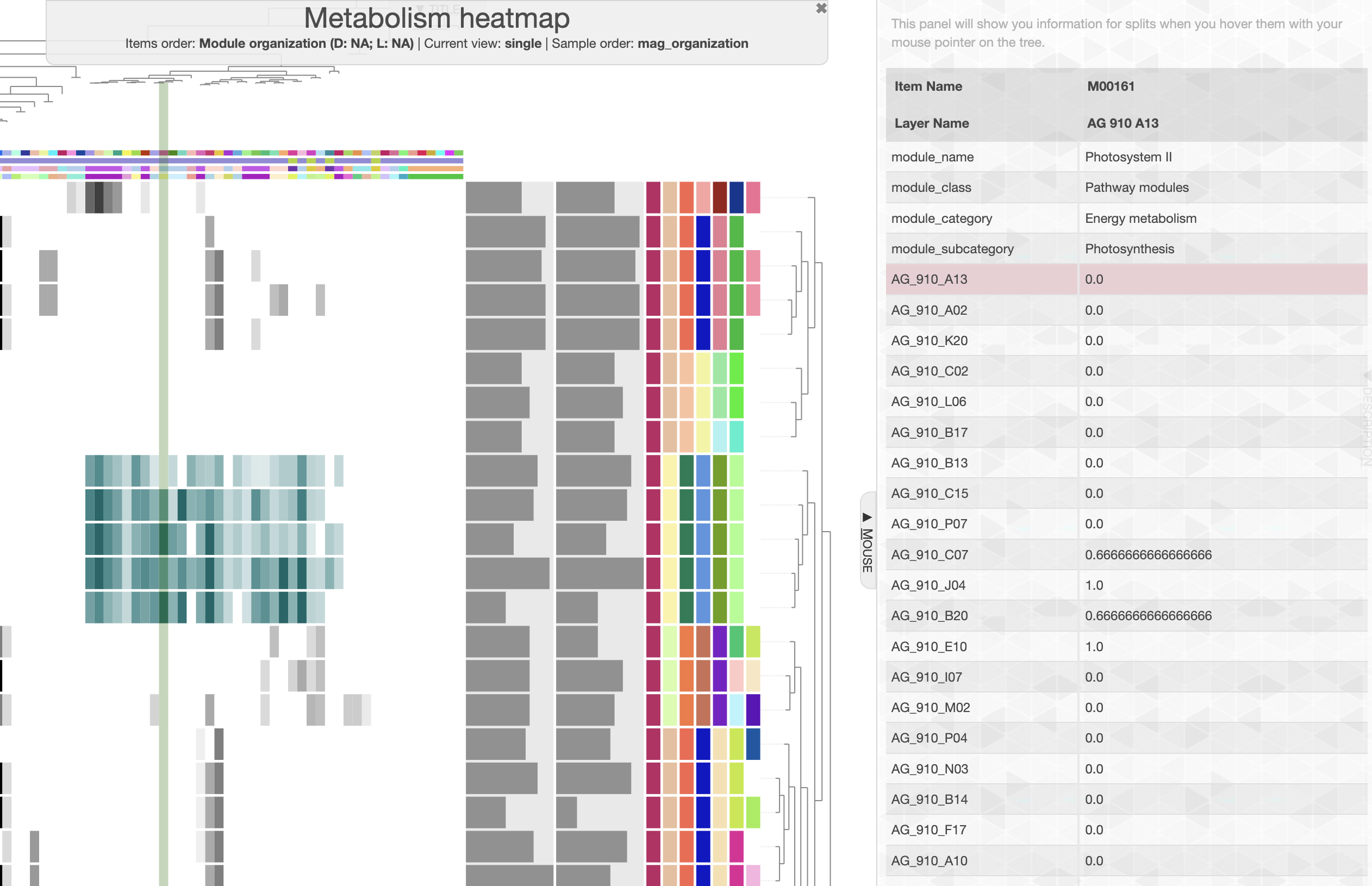
In the main panel, you can change the “Items order” to “Module organization” and in the layer panel, you can now choose to order by “SAG_organization”. And here is what you should be able to see:
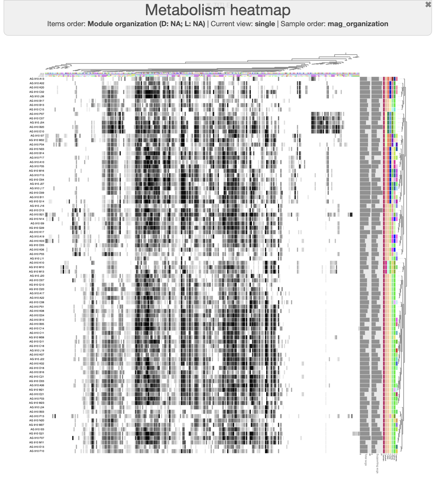
We can easily see a cluster of 5 SAGs, which possess a distinctive group of module. If you change the module name layer from color to text, or if you use the “mouse” panel and hover over the corresponding module, you will see module like “Photosystem II” and other electron transfer pathways that likely indicate that these SAGs are Cyanobacteria. And if you look at the taxonomy data on the right side of the heatmap, you will see that indeed these 5 SAGs are assigned to the Prochlorococcus genus.
User defined pathways
Are you familiar with the marine methane paradox? Because I didn’t know about it before writing this tutorial. I learn about is while reading this paper by Carini et al. 2014. Basically, methane is actually supersaturated in the surface ocean compared to the atmosphere, and it is due to biological activity. Methylphosphonic acid is produced by marine archaea and under phosphate limitation, some bacteria like Pelagibacter are able to uptake and process methylphosphonic acid which releases methane. Two operons have been identified for the transport and process of methylphosphonic acid: PhnCDEE and PhnGHIJKLNM.
At the very beginning of this tutorial, we visually inspected a SAG and we looked for the phosphate transporter operon (pstSCAB). So now we have three operons for two types of phosphate uptake and utilization. These genes are annotated by KEGG (and COG) but are not part of the KEGG’s module and we cannot simply search for the completeness of these transporters in the default output of anvi-estimate-metabolism. Fortunately for us, we can create our own metabolism module in anvi’o and use anvi-estimate-metabolism to get the completeness and copy number of a user-defined metabolic module.
Let’s create three user-defined module/pathway for the three operons pstSCAB, PhnCDEE and PhnGHIJKLNM. At the moment, the user-defined module in anvi’o follow the same (annoying) structure as KEGG module. We need to create three files, one for each module. Use your favorite text editor and create the following file:
pstSCAB.txt
ENTRY       pstSCAB
NAME        Pi Transport
DEFINITION  COG0226 COG0573 COG0581 COG1117
ORTHOLOGY   COG0226  pstS
            COG0573  pstC
            COG0581  pstA
            COG1117  pstB
CLASS       User modules; Transport System; Pi Transport
ANNOTATION_SOURCE  COG0226  COG20_FUNCTION
                   COG0573  COG20_FUNCTION
                   COG0581  COG20_FUNCTION
                   COG1117  COG20_FUNCTION
///
PhnCDE.txt
ENTRY       PhnCDEE
NAME        Organophosphorus Transport
DEFINITION  COG3638 COG3221 COG3639
ORTHOLOGY   COG3638  PhnC
            COG3221  PhnD
            COG3639  PhnE
CLASS       User modules; Transport System; Organophosphorus Transport
ANNOTATION_SOURCE   COG3638  COG20_FUNCTION
                    COG3221  COG20_FUNCTION
                    COG3639  COG20_FUNCTION
///
PhnGHIJKLNM.txt
ENTRY       PhnGHIJKLNM
NAME        Phosphonate Utilization
DEFINITION  COG3624 COG3625 COG3626 COG3627 COG4107 COG4778 COG3709 COG3454
ORTHOLOGY   COG3624  PhnG
            COG3625  PhnH
            COG3626  PhnI
            COG3627  PhnJ
            COG4107  PhnK
            COG4778  PhnL
            COG3709  PhnN
            COG3454  PhnM
CLASS       User modules; Transport System; Phosphonate Utilization
ANNOTATION_SOURCE   COG3624  COG20_FUNCTION
                    COG3625  COG20_FUNCTION
                    COG3626  COG20_FUNCTION
                    COG3627  COG20_FUNCTION
                    COG4107  COG20_FUNCTION
                    COG4778  COG20_FUNCTION
                    COG3709  COG20_FUNCTION
                    COG3454  COG20_FUNCTION
///
Now we need to setup these module so we can use them in anvi’o using anvi-setup-user-modules. For that we need to create a special directory structure:
mkdir CUSTOM_PATHWAYS
mkdir CUSTOM_PATHWAYS/modules
mv pstSCAB.txt CUSTOM_PATHWAYS/modules/
mv PhnCDE.txt CUSTOM_PATHWAYS/modules/
mv PhnGHIJKLNM.txt CUSTOM_PATHWAYS/modules/
Then we can run anvi-setup-user-modules, which will generate a modules-db:
anvi-setup-user-modules -u CUSTOM_PATHWAYS/
Finally, we can use external-genomes with our user-defined module and investigate the presence and completeness of our phosphate transport among all the SAGs with a minimum of 50% completion estimation:
anvi-estimate-metabolism -e external-genomes-50.txt \
                         -O phostphate-transporter \
                         -u CUSTOM_PATHWAYS/ \
                         --only-user-modules
At the beginning of the tutorial, we looked at SAG AG-910-K02 and in the output files we can see that the pstSCAB transporter is indeed complete, but that SAG does not have the methylphosphonic acid transporter. Difficult to say if it is truly lacking the transporter or if it is a limitation of an incomplete SAG.
| module | genome_name | db_name | module_name | module_class | module_category | module_subcategory | module_definition | stepwise_module_completeness | stepwise_module_is_complete | pathwise_module_completeness | pathwise_module_is_complete | proportion_unique_enzymes_present | enzymes_unique_to_module | unique_enzymes_hit_counts | enzyme_hits_in_module | gene_caller_ids_in_module | warnings |
|---|---|---|---|---|---|---|---|---|---|---|---|---|---|---|---|---|---|
| pstSCAB.txt | AG_910_K02 | AG_910_K02 | Pi Transport | User modules | Transport System | Pi Transport | “COG0226 COG0573 COG0581 COG1117” | 1.0 | True | 1.0 | True | 1.0 | COG0226,COG0573,COG0581,COG1117 | 1,1,1,1 | COG0226,COG0573,COG0581,COG1117 | 745,744,743,742 | None |
The SAG AG-910-F07 is also a Pelagibacter like AG-910-K02, and it has both transporter:
| module | genome_name | db_name | module_name | module_class | module_category | module_subcategory | module_definition | stepwise_module_completeness | stepwise_module_is_complete | pathwise_module_completeness | pathwise_module_is_complete | proportion_unique_enzymes_present | enzymes_unique_to_module | unique_enzymes_hit_counts | enzyme_hits_in_module | gene_caller_ids_in_module | warnings |
|---|---|---|---|---|---|---|---|---|---|---|---|---|---|---|---|---|---|
| pstSCAB.txt | AG_910_F07 | AG_910_F07 | Pi Transport | User modules | Transport System | Pi Transport | “COG0226 COG0573 COG0581 COG1117” | 1.0 | True | 1.0 | True | 1.0 | COG0226,COG0573,COG0581,COG1117 | 1,1,1,1 | COG0226,COG0573,COG0581,COG1117 | 886,887,888,889 | None |
| PhnGHIJKLNM.txt | AG_910_F07 | AG_910_F07 | Phosphonate Utilization | User modules | Transport System | Phosphonate Utilization | “COG3624 COG3625 COG3626 COG3627 COG4107 COG4778 COG3709 COG3454” | 1.0 | True | 1.0 | True | 1.0 | COG3454,COG3624,COG3625,COG3626,COG3627,COG3709,COG4107,COG4778 | 1,1,1,1,1,1,1,1 | COG3454,COG3624,COG3625,COG3626,COG3627,COG3709,COG4107,COG4778 | 334,326,327,328,329,332,330,331 | None |
| PhnCDE.txt | AG_910_F07 | AG_910_F07 | Organophosphorus Transport | User modules | Transport System | Organophosphorus Transport | “COG3638 COG3221 COG3639” | 1.0 | True | 1.0 | True | 1.0 | COG3221,COG3638,COG3639 | 1,1,2 | COG3221,COG3638,COG3639,COG3639 | 323,324,321,322 | None |
This output file will be very interesting later as we will generate a pangenome of SAR11 SAGs and we can decorate that pangenome with the presence/absence of the transporter and discuss its evolutionary distribution in SAR11.
More?
Once you have multiple contigs-db for each SAG, you can use any anvi’o program that uses an external-genomes as an input. You can look at the anvi’o help page for the external-genomes to see which program can use it. For instance, you can compute the functional enrichment between groups of genomes with anvi-compute-functional-enrichment-across-genomes; or compute codon usage bias with anvi-get-codon-usage-bias.
You can also use the command anvi-script-gen-hmm-hits-matrix-across-genomes and anvi-get-sequences-for-hmm-hits to find conserved genes across multiple genomes, a required step to compute a phylogenomic tree.
Phylogenomics
Another way to investigate the microbial diversity of these SAGs is to create a phylogenomic tree using a single-copy core genes, like ribosomal proteins.
Find most prevalent ribosomal protein genes
We need to look into the distribution of ribosomal proteins across all SAG to choose which genes are the most suitable for our phylogenomic tree. We can use the command anvi-script-gen-hmm-hits-matrix-across-genomes, which uses an external-genomes for input.
I also want to constrain this tree to only SAG with a completion estimate above 50%. We need to make a new external-genomes that only contains SAGs with >50% completion:
# search for SAGs >50% completion and get their name in a file
awk '$4>50{print $1}' completion-redundancy.txt > 50_completion_SAGs.txt

# subset external-genomes.txt for the SAGs of interest
head -n 1 external-genomes.txt > external-genomes-50.txt
grep -f 50_completion_SAGs.txt external-genomes.txt >> external-genomes-50.txt
Now we can use anvi-script-gen-hmm-hits-matrix-across-genomes:
anvi-script-gen-hmm-hits-matrix-across-genomes -e external-genomes-50.txt \
                                               --hmm-source Bacteria_71 \
                                               -o hmm_matrix.txt
I don’t like the orientation of this matrix, but we can transpose it and look for the most prevalent ribosomal protein:
anvi-script-transpose-matrix hmm_matrix.txt \
                             -o hmm_matrix_transpose.txt

# the awk command sum the frequency of each SCG
awk 'NR>1{for(i=2;i<=NF;i++) if($i>0){t+=1}; print $1"\t"t; t=0}' hmm_matrix_transpose.txt | grep -i ribosom | sort -nrk2 | head -n 10
Here are the 10 most prevalent ribosomal proteins:
Ribosomal_S3_C	76
Ribosomal_L27A	76
Ribosomal_S19	75
Ribosomal_L22	75
Ribosomal_S13	74
Ribosomal_S11	74
Ribosomal_L2	74
Ribosomal_L16	74
Ribosomal_S8	73
Ribosomal_L6	73
Make a tree from ribosomal proteins
The first step is to get the amino acid sequence for the ribosomal proteins that we have just selected. We can use the program anvi-get-sequences-for-hmm-hits, which is used to do exactly what it says: get the sequence of genes matching an HMM collection. When using the flag --concatenate-genes, the program will not simply give you the sequence for each genes, but it will concatenate all the genes per genome and later generate a multiple sequences alignment using Muscle. We also need to specify which HMM source we want to use and the name of the genes of interest.
# make a directory to store the results
mkdir -p PHYLOGENOMICS

# run the command
anvi-get-sequences-for-hmm-hits -e external-genomes-50.txt \
                                --hmm-source Bacteria_71 \
                                --gene-names Ribosomal_S3_C,Ribosomal_L27A,Ribosomal_S19,Ribosomal_L22,Ribosomal_S13,Ribosomal_S11,Ribosomal_L2,Ribosomal_L16,Ribosomal_S8,Ribosomal_L6 \
                                --get-aa-sequences \
                                --concatenate-genes \
                                --max-num-genes-missing-from-bin 2 \
                                --return-best-hit \
                                -o PHYLOGENOMICS/ribosomal_proteins.fa
Some SAGs will be missing some of our genes of interest, it will create big gaps in the multiple sequence alignment but that is ok. We don’t want to miss out on a SAG that is missing one ribosomal protein in our list, but we don’t to include SAGs with only one genes. That’s why we use the flag --max-num-genes-missing-from-bin 2, which will filter out SAGs missing more than 2 genes from our list of ribosomal protein. After running the command you will see that 71/81 SAGs had at least 8 of the 10 ribosomal genes from our list and will remain in the final tree.
Now we need to make a tree. There are multiple option outside of anvi’o at this stage, so you could use your favorite tree making program and skip this step. For now we will use anvi-gen-phylogenomic-tree, which uses FastTree.
anvi-gen-phylogenomic-tree -f PHYLOGENOMICS/ribosomal_proteins.fa \
                           -o PHYLOGENOMICS/ribosomal_proteins.tree
Congrats, you have a newick tree!
Visualize the phylogenomic tree
We can use anvi-interactive to visualize any newick tree. For that we need to use the --manual mode. The program still requires a profile-db to store any changes you make in the interactive interface. But no worries, anvi’o will create it for you:
anvi-interactive -t PHYLOGENOMICS/ribosomal_proteins.tree \
-p PHYLOGENOMICS/profile.db \
--manual \
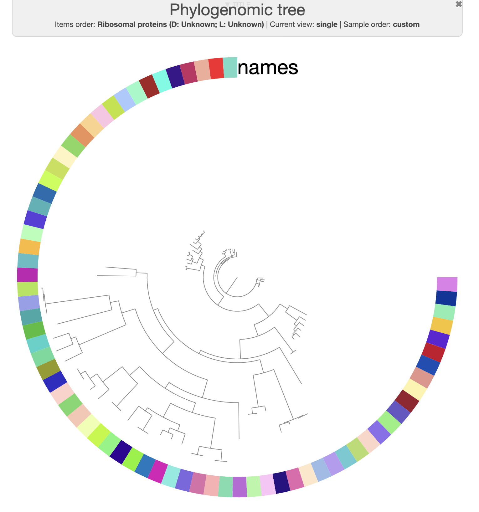
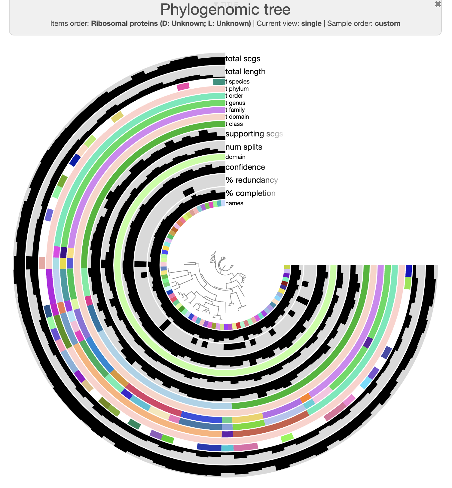
--title "Phylogenomic tree"
Click the draw button and you should see this
You can play with the interface and adjust the setting until you have the figure of your dreams. The tree is not rooted, but you can right-click a single branch (or ctrl+right-click for a group of branch) and root the three from there (or just rotate the tree). But where should we root this tree? To help us, we can add the taxonomic information that we generated earlier. Let’s close the webpage, go back to the terminal and press ctrl+c to close the stop the anvi-interactive command.
To add additional information for item on the interface, we can use anvi-interactive with the flag -A. Or better, since we generated a profile-db with the previous command, we can add the taxonomy information directly in it with anvi-import-misc-data. And while we are doing that, we might as well import the completeness/redundancy estimates:
anvi-import-misc-data -p PHYLOGENOMICS/profile.db -t items taxonomy.txt
anvi-import-misc-data -p PHYLOGENOMICS/profile.db -t items completion-redundancy.txt
Now the interactive interface again:
anvi-interactive -t PHYLOGENOMICS/ribosomal_proteins.tree \
                 -p PHYLOGENOMICS/profile.db \
                 --manual \
                 --title "Phylogenomic tree"
If you open the Mouse panel on the right side and then hover your mouse over the figure, you can see the value of any data under your mouse on the display, including the taxonomic annotation.
You can play with multiple setting in the interactive interface. For instance, here is how my tree looks like after a few min of tinkering around and rooting with the three cyanobacteria SAGs:
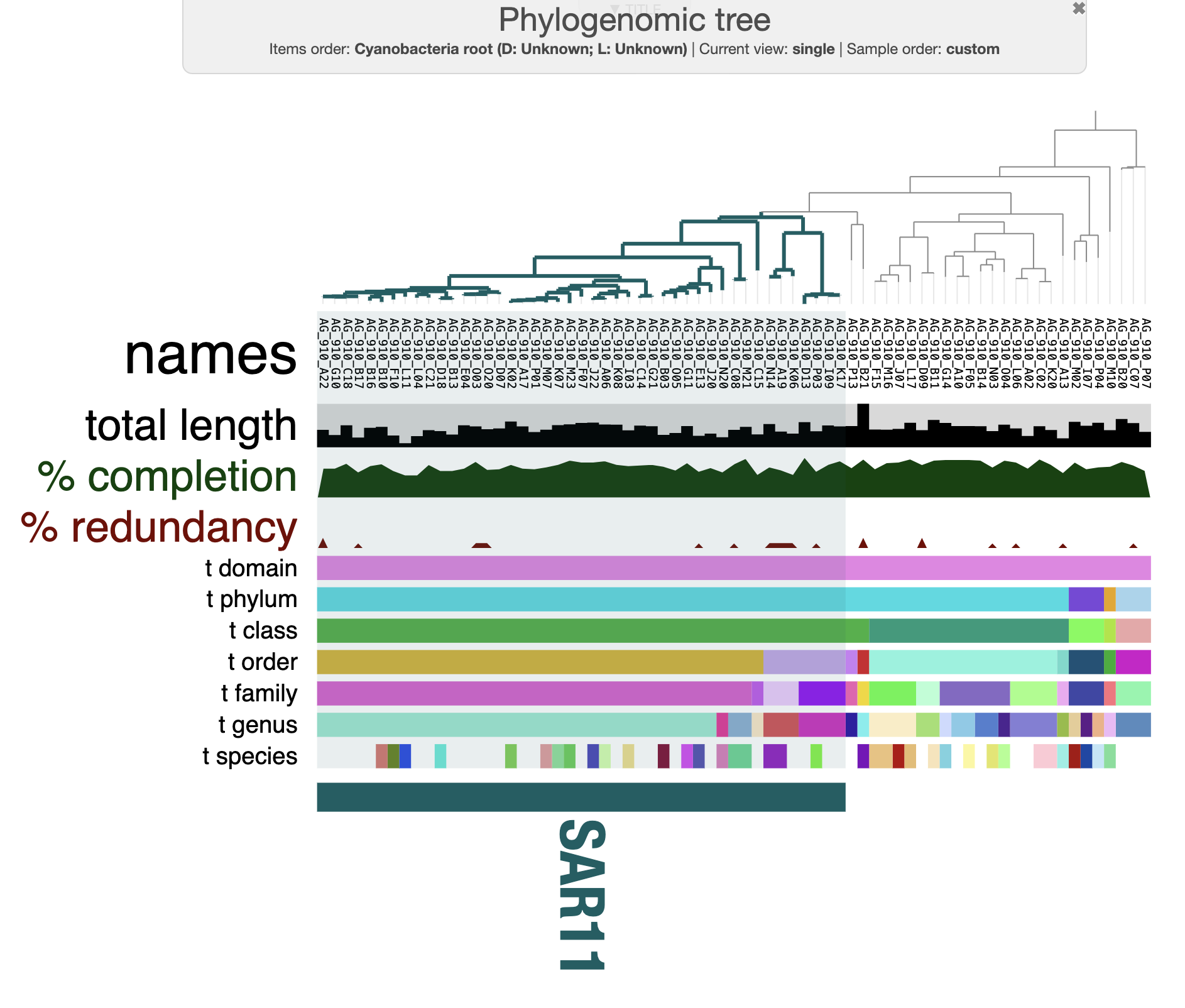
If you choose to root your tree in the interface, don’t forget to save the rooted tree in the “Main” panel, just under the “item order” drop down menu.
You can choose to display branch support values on your tree but there is a well-known issue with tree branch support values not properly placed after rooting a tree in some tree software, including anvi’o v8. If you are using a more recent version of anvi’o or the development branch, this issue has been fixed. You can check this github issue to learn more about it.
Don’t forget to save the “state” of your figure before closing the interface. All the settings, colors, etc, are stored in the profile-db. Anyone with anvi’o would be able to use that profile-db and see the figure you made and make modification, save, and share again. Best, you can upload the profile-db and the tree file to an open repository like figshare or zenodo, reference them in your manuscript to allow readers to reproduce your results and figures.
You can export the figure from the interactive interface by clicking on the save icon button. It will generate an SVG file that you can edit in your favorite vector graphics software (*cough* inkscape and you are ready for publication.
A next step is to compare the SAGs to each other. In other words - we will do some comparative genomics by comparing their gene content (pangenomics), compute genome similarity, and a bit more. We can see that the majority of SAGs present on this tree belong to the SAR11 groups. In the next part of the tutorial we will dive into comparative genomics to understand how these genomes related to each others.
Pangenomics
In pangenomics, we examine the distribution of genes across genomes. Genes that are present in all genomes in the analysis are known as ‘core genes’, while genes that appear in only a subset of the genomes are called ‘accessory genes’. A third category is singleton gene cluster that are only present in one genome.
For our pangenome analysis, we will focus on a set of SAGs from the SAR11 clade (Pelagibacterales and HIMB59 orders). Here is the list of all SAGs from these orders with a minimum completion estimate of 75%:
AG_910_A06  AG_910_F07  AG_910_K08
AG_910_B10  AG_910_G11  AG_910_K17
AG_910_C08  AG_910_G21  AG_910_M21
AG_910_C14  AG_910_I09  AG_910_M23
AG_910_C18  AG_910_J22  AG_910_O03
AG_910_C21  AG_910_K02
AG_910_D13  AG_910_K07
To add some context in this comparative genomic approach, we can add some reference genomes. In the directory ADDITIONAL_DATA, you will find two contigs databases which were generated with the genomes of HIMB083 and HIMB59.
In the datapack, there is a new external genomes file which only includes the list of selected SAGs and the two reference genomes. Let’s copy it to our working directory:
cp ADDITIONAL_DATA/external-genomes-pangenomics.txt .
Download and include NCBI genomes in anvi’o We often need to include genomes from public repositories to generate better comparisons. One common resource is NCBI. Here is a comprehensive tutorial on how to obtain NCBI genomes with anvi’o.
In brief, you can install and use the program ncbi-genome-download to get genomes from GenBank or RefSeq. It is very flexible: you can search for complete or draft genomes, specify genomes using their taxids, or ask for all genomes from a given genera, etc.
Then you can use the program anvi-script-process-genbank-metadata which takes the output of ncbi-genome-download to generate FASTA files, external gene calls files and functional annotation files. It also creates a fasta-txt file, which can directly be used by anvi-run-workflow to generate contigs databases.
Genome storage
A genomes-storage database is a special anvi’o database to store genome information. To create a genomes storage with the genomes from the list above, we can use the command anvi-gen-genomes-storage along with the new external genomes file:
# create a directory to store the pagenomics databases
mkdir -p PANGENOMICS

# create the genomes storage db
anvi-gen-genomes-storage -e external-genomes-pangenomics.txt \
                         -o PANGENOMICS/SAR11-GENOMES.db
Success? Good.
Pangenome analysis
Once your genomes storage is ready, you can use anvi-pan-genome to run the actual analysis:
anvi-pan-genome -g PANGENOMICS/SAR11-GENOMES.db \
                -n SAR11 \
                -o PANGENOMICS\
                -T 4
In brief, when you use this program, anvi’o will use DIAMOND to compute the similarity between each amino acid sequence in every genome. Then, it uses the MCL algorithm to identify clusters in the amino acid similarity search results. Here you can find more information about the parameters of anvi-pan-genome.
Display the pangenome
When the analysis is done, you can use anvi-display-pan to start an interactive web page containing the results:
anvi-display-pan -g PANGENOMICS/SAR11-GENOMES.db \
                 -p PANGENOMICS/SAR11-PAN.db
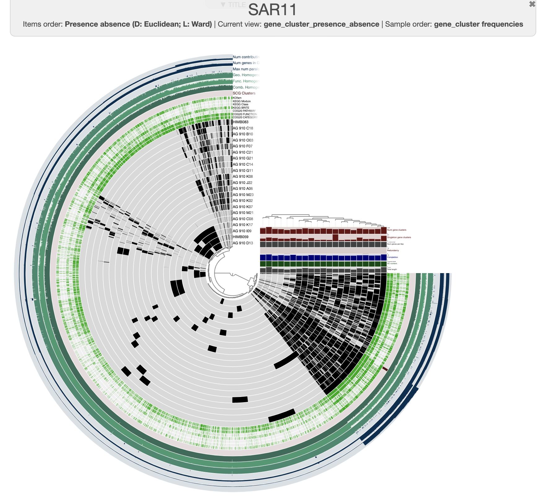
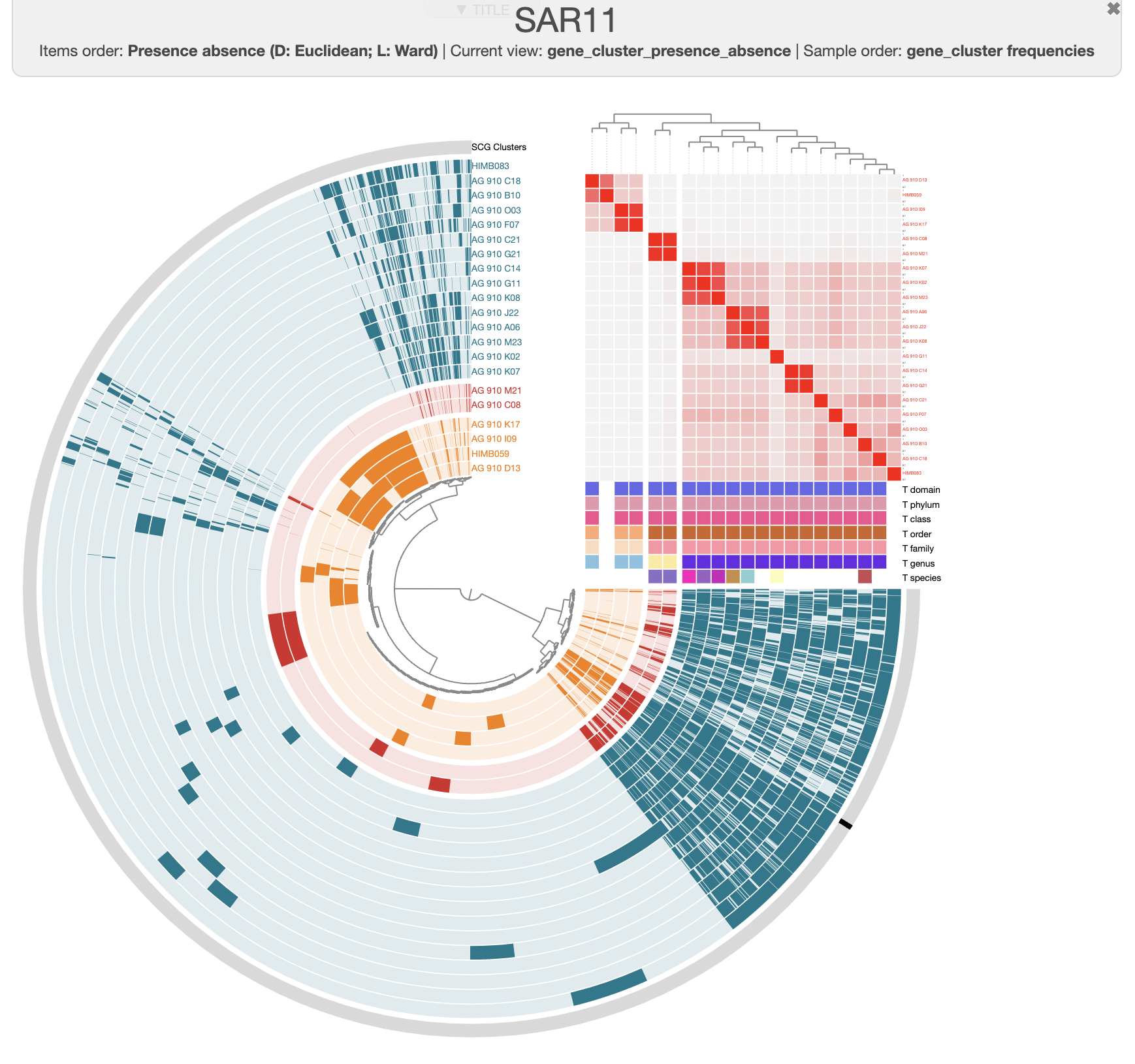
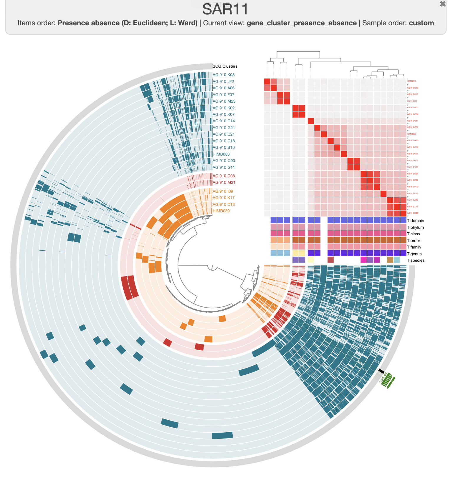
This is what you should see when you click the Draw button:
It is pretty messy at the moment. To improve it, you can order the genomes based on the gene clusters’ distribution by selecting the gene cluster frequencies tree from the Samples panel and Sample Order menu:
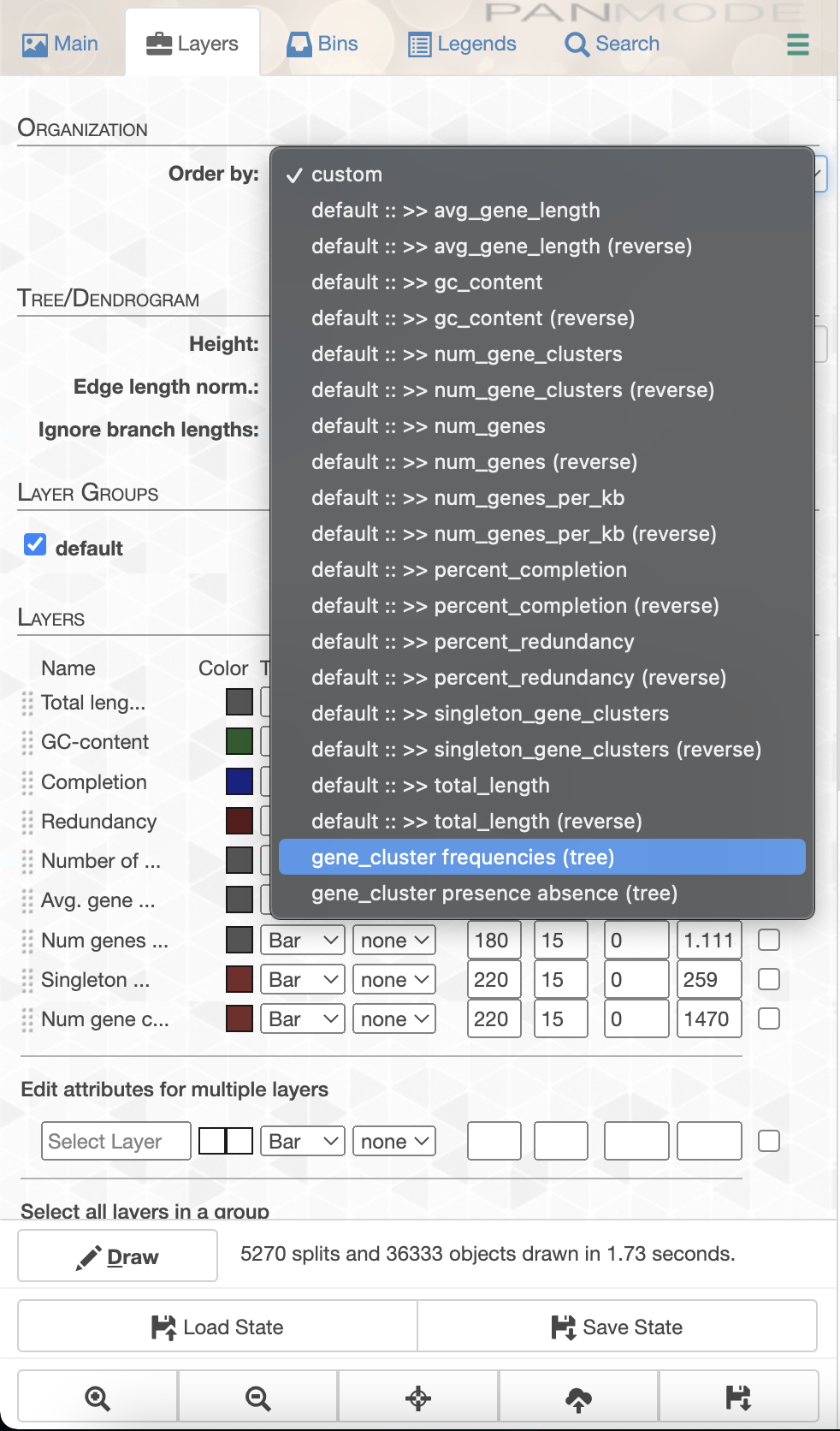
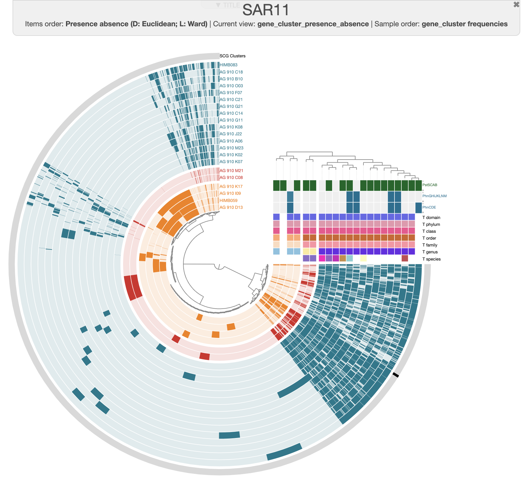
And this is what you should see when you draw again:
It is a bit more organized. You can save the current state in the main panel. Every time you will start this interactive interface, it will load the default state. For now, let’s close it and kill the server. We can add some meaningful information onto it, like the taxonomy of each of these SAGs! To do that, we can use the command anvi-import-misc-data. Right now, we have the file taxonomy.txt which has taxonomy information for all 228 of the SAGs, and anvi’o would be upset if we tried to import this table for a pangenome of only 21 genomes. But it is ok, we can use the flag --just-do-it and anvi’o will try its best.
anvi-import-misc-data -p PANGENOMICS/SAR11-PAN.db \
                      -t layers \
                      --just-do-it \
                      taxonomy.txt
You can rerun anvi-display-pan and take some time to explore the Main and Layers panels to modify some aesthetics.
anvi-display-pan -g PANGENOMICS/SAR11-GENOMES.db \
                 -p PANGENOMICS/SAR11-PAN.db
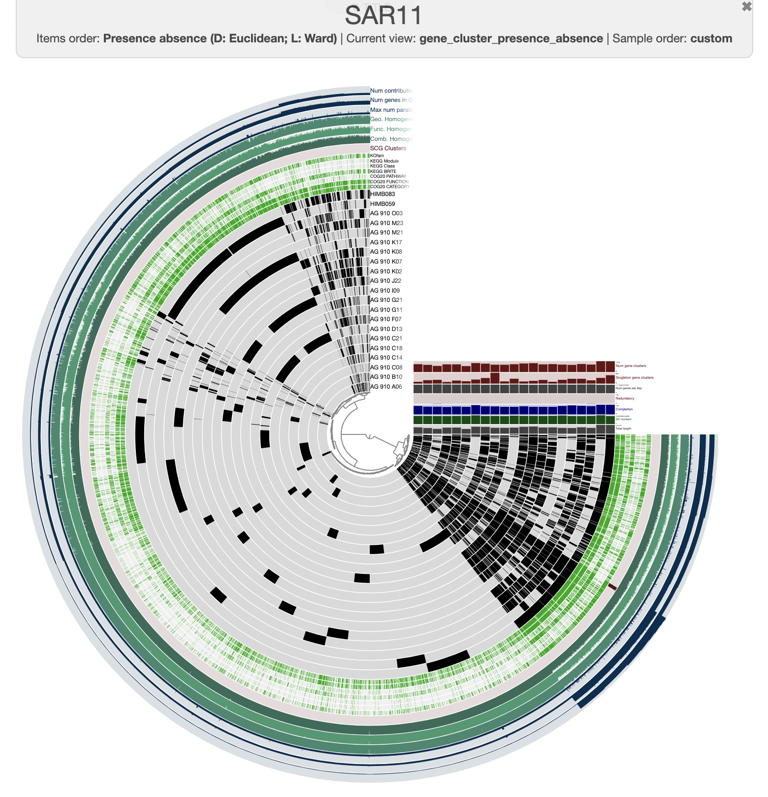
For instance, this is the same pangenome, just prettier:
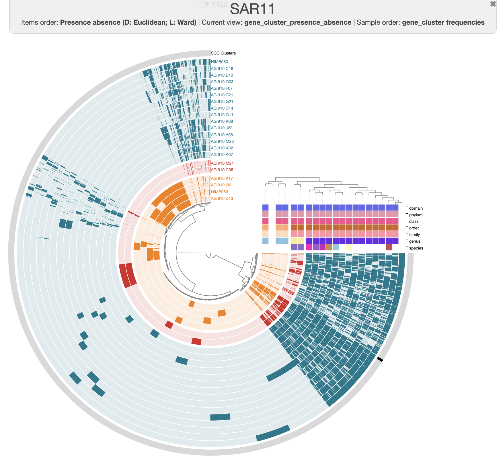
You can export the figure as an SVG with the save button on the bottom of the setting panel and use your favorite SVG-eating software like Inkscape.
There are three distinct groups of SAGs and reference genomes based on their gene content. Each group also has consistent taxonomy annotations, with the blue group (in the figure above) belonging to HIMB59, the red containing Pelagibacter genomes, and the green group has two GCA-002704185 sp902517865 genomes, which are members of the Pelagibacterales.
Bin gene clusters and summarize the pangenomic analysis
A gene cluster can be part of the ‘core’ genome when it is shared by all the genomes, or part of the ‘accessory’ genome of a subset of genomes. Finally, if a gene cluster is only found in one genome, then we usually refers to it as a ‘singleton’ gene cluster. If you are interested in the set of genes that are unique to a subgroup, or to a single genome, you can use the interactive interface to ‘bin’ gene clusters and later summarize these bins to obtain the amino acid sequences of these genes and their functions.
To create a bin, you can simply click on gene clusters and they will be added to the current bin. A more efficient way to add gene clusters to a bin is to click on branches in the central dendrogram.
You can use the Bin tab to select, rename, and create bins.
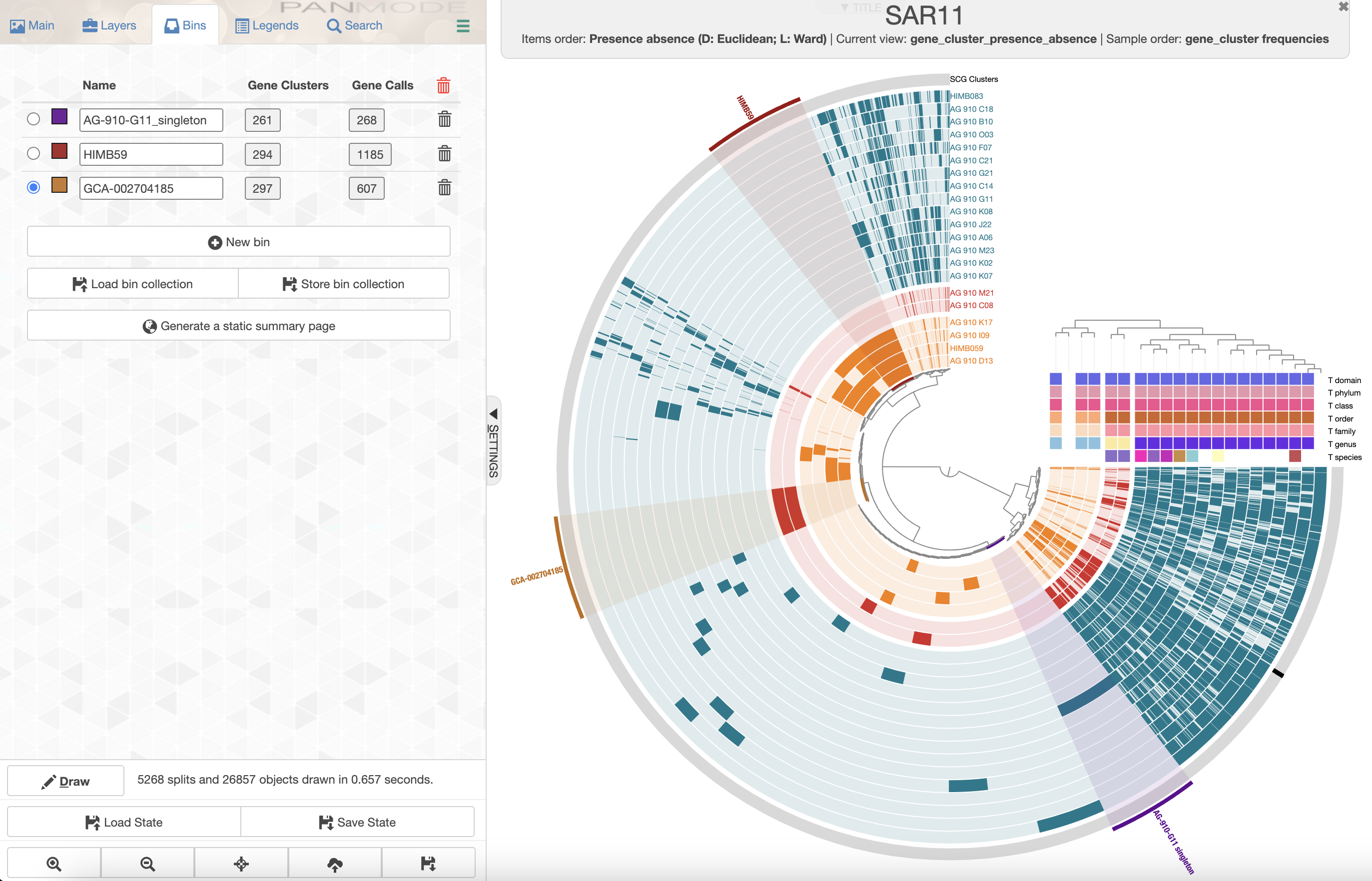
Let’s select the accessory genomes of GCA-002704185 sp902517865 and HIMB59, and also select the singleton gene clusters of AG-910-G11 to further inspect these genes and therefore the functions that make these genomes unique compared to the rest.
After selecting branches on the dendrogram, and renaming the bins, you should have a figure that looks somewhat like this:
You can have a quick look at the content of a bin by clicking on the box with the number of gene clusters.
You can store the collection of bins by clicking on the “Store bin collection” button. Anvi’o lets you make as many collections of bins as you want. You can give the collection a meaningful name, but for now we can just save it as default.
A better way to inspect these bins is to use the program anvi-summarize. Kill the interactive interface and run the following command:
anvi-summarize -g PANGENOMICS/SAR11-GENOMES.db \
               -p PANGENOMICS/SAR11-PAN.db \
               -C default \
               -o SUMMARY
It will create the directory SUMMARY, which contains the file SAR11_gene_clusters_summary.txt.gz. To decompress this file, you can run:
gunzip SUMMARY/SAR11_gene_clusters_summary.txt.gz
Now you have a TAB-delimited file with all the genes occurring in the entire pangenome. There is also a column called bin_name to help you investigate the genes unique to GCA-002704185 sp902517865, HIMB59, and AG-910-G11.
Compute average nucleotide identity
A common metric used to compare genomes is the average nucleotide identity (ANI). Anvi’o has a program, anvi-compute-genome-similarity, which uses different similarity metrics to compute ANI across your SAGs. It is a convenient program that can accept the external genomes file and optionally a pan-db to display the result directly on top of the pangenome figure. Today, we will run PyANI using this program.
Here is how to run the command:
anvi-compute-genome-similarity -e external-genomes-pangenomics.txt \
                               -p PANGENOMICS/SAR11-PAN.db \
                               -o ANI \
                               --program pyANI \
                               -T 4
Once this is complete, we can visualize the pangenome with anvi-display-pan.
anvi-display-pan -g PANGENOMICS/SAR11-GENOMES.db \
                 -p PANGENOMICS/SAR11-PAN.db
At first, there is nothing new. But if you go in the Layers tab, you will see this:
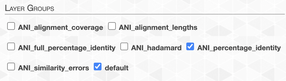
Select ANI_percentage_identity and click on Redraw layer data. Then you should see the ANI on the display.
You probably want to change the min value from the interface to better appreciate the differences in the ANI heatmap across all the genomes.
You can now also organize the genomes based on the ANI value using the menu Order by in the Layers tab.
We can learn a few things with this analysis so far. First of all, AG-910-D13 is quite closely related to the reference genome HIMB59. Second of all, AG-910-G11 is still part of the of the same cluster as all the other Pelagibacter genomes, but it is clearly more different with a low ANI compare to the other genomes.
Order genomes based on SCGs similarity
We compared genomes using their gene content and ANI, we can also used a collection of shared genes to create a phylogenomic tree. With the pangenome, we have access to shared genes that are specific to that group. We can use them instead of the bacterial SCGs and investigate if the cluster of genomes observed with the previous two approaches can be found in the evolution of shared genes. Note that this approach is not what you would do for phylogenomic tree where you want to show evolutionary relationship in the tree of life. For that you would need to use appropriate genes like ribosomal protein and include an out-group for rooting.
Let’s make a phylogenomic tree of the 21 genomes we used in the pangenomic analysis.
We can use anvi-get-sequences-for-hmm-hits like we did for the phylogenomic analysis. But in closely-related genomes, some single-copy core genes will be 100% similar across all genomes. If we include them in the alignment, they will not contribute to to the phylogenomic signal. In addition, we don’t need to use the small set of bacterial single-copy core genes when we can use the ‘core’ genome specific to our small set of Pelagibacterales.
In the pangenomic analysis, anvi’o computes two metrics for each gene cluster: functional homogeneity and geometric homogeneity. Because not all gene clusters are created equal, we use these metrics to distinguish very homogeneous gene clusters with very high amino acid sequence similarity from less homogeneous one with divergent amino acid sequences. The latter category would be interesting to use for a phylogenomic analysis.
Geometric homogeneity indicates the degree of geometric configuration between the genes of a gene cluster. Basically, it takes into account the gap/residue pattern. Functional homogeneity uses the aligned residues and attempts to quantify their differences considering the biochemical properties of amino acids, which would affect gene structure/function.
Filter gene clusters
To select a suitable set of genes, we can use the pangenome interface. If you closed it, you can run:
anvi-display-pan -g PANGENOMICS/SAR11-GENOMES.db \
                 -p PANGENOMICS/SAR11-PAN.db
You can filter for specific gene clusters using the Search tab and the Search gene clusters using filters section:
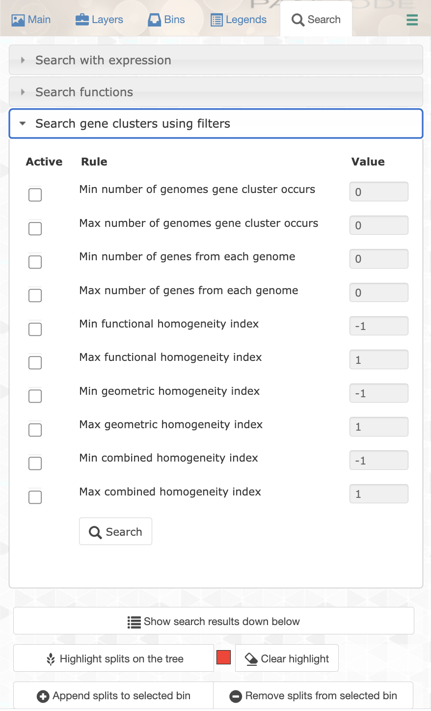
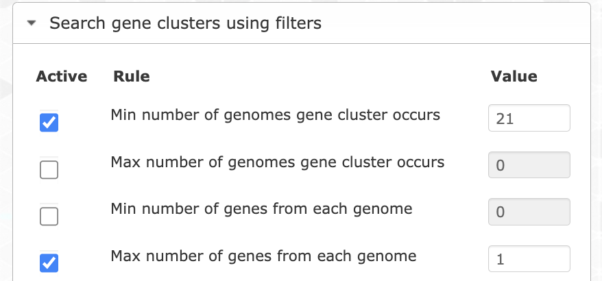
Let’s try different filters to find the best set of genes. We can start by choosing only the single-copy core gene clusters. For that you want to filter for gene clusters occurring in all genomes (min 21), and with a maximum of 1 gene per genome.
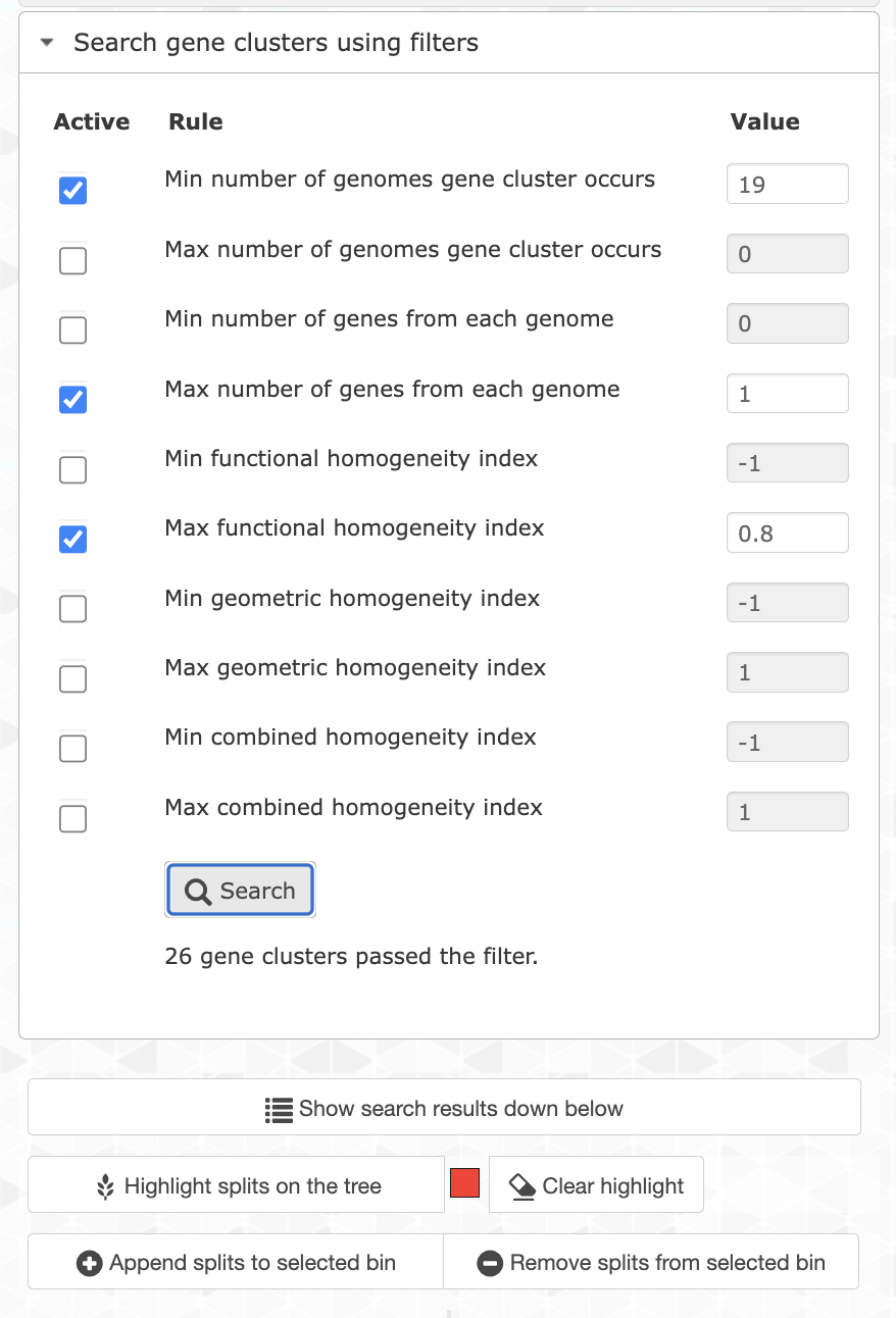
If you search for them and highlight the results on the tree, you will see that they correspond to the ‘SCG cluster’ layer, which makes total sense. That’s 13 gene clusters, which is not a lot. Unfortunately the core genome is pretty small in this pangenome, which is likely due to the fragmented nature of the SAGs. So we can be a little bit more flexible and search for gene clusters occurring in at least 19 out of 21 genomes by changing the appropriate filter. We can also filter for less homogeneous gene clusters to keep only the most divergent ones (max functional homogeneity of 0.8):
You can now add these gene clusters to a bin (make sure you’re using an empty bin or create a new one in the Bin tab) by clicking on the button Append splits to selected bin.
Compute and display the phylogenomic tree
Now to make the alignment and the phylogenomic tree, you can simply navigate to the Layers tab where you will see a button Generate a new phylogenetic tree. When you click on it you can name your tree, select the bin you have just made, choose an aligner, and finally check the box to store the tree permanently.
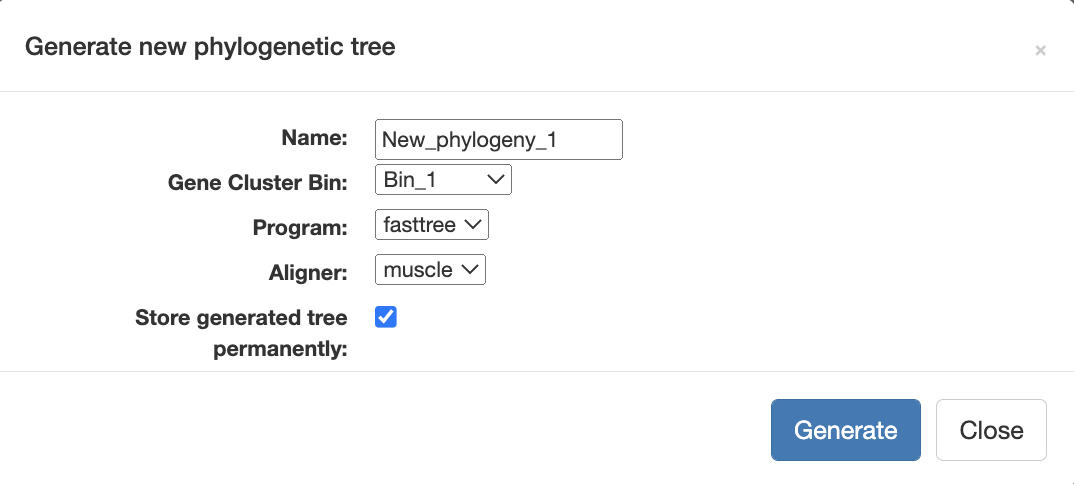
Anvi’o will automatically display the tree and reorganize the genomes accordingly:
Unsurprisingly, we can still see three clusters corresponding to the three genera, and these clusters fit well with the ANI heatmap. Notice how AG-910-G11 is now more outside of the Pelagibacter cluster than we previously observed?
Make a phylogenomic tree outside of the interactive interface
You don’t need to use the interactive interface to extract, align, and compute a phylogenomic tree. Instead, you can use the program anvi-get-sequences-for-gene-clusters. It accepts a genome storage and a pan db, and you can use the same filters as the ones in the Search tab of the interactive interface. For instance, this command would give you the same set of genes as a multiple sequence alignment:
anvi-get-sequences-for-gene-clusters -g PANGENOMICS/SAR11-GENOMES.db \
                                     -p PANGENOMICS/SAR11-PAN.db \
                                     -o concatenated-proteins-SAR11.fa \
                                     --concatenate-gene-clusters \
                                     --min-num-genomes-gene-cluster-occurs 19 \
                                     --max-num-genes-from-each-genome 1 \
                                     --max-functional-homogeneity-index 0.8
You can then compute a tree with anvi-gen-phylogenomic-tree:
anvi-gen-phylogenomic-tree -f concatenated-proteins-SAR11.fa \
                           -o phylogenomic-tree-SAR11.txt
And use anvi-interactive to display the tree:
anvi-interactive -p phylogenomic-profile-SAR11.db \
                 -t phylogenomic-tree-SAR11.txt \
                 --title "Phylogenomic_tree_SAR11" \
                 -A taxonomy.txt \
                 --manual
You can always import that tree into an existing pangenome with anvi-import-misc-data, but you will need to reformat the tree to fit the input format - click here to learn more.
Exploratory analysis: phosphate transporters
Following up to the [earlier section of this tutorial] where we created user-defined module for two phosphate transporters and utilization operons, we can run anvi-estimate-metabolism again using the external-genomes external-genomes-pangenomics.txt (which includes the two reference genomes). And then display the result on the pangenome itself:
anvi-estimate-metabolism -e external-genomes-pangenomics.txt \
                         -O phostphate-transporter-pan \
                         -u CUSTOM_PATHWAYS/ \
                         --matrix-format \
                         --only-user-modules
We need to reformat the data a little bit, and then we can import it in our pangenome database:
anvi-script-transpose-matrix phostphate-transporter-pan-module_pathwise_completeness-MATRIX.txt \
                             -o phostphate-transporter-layers.txt
# replace the header "module" to "layers"
sed 's/module/layers/' phostphate-transporter-layers.txt > tmp && mv tmp phostphate-transporter-layers.txt
# rename the module's names
sed 's/\.txt//g' phostphate-transporter-layers.txt > tmp && mv tmp phostphate-transporter-layers.txt
# import the layers data
anvi-import-misc-data -p PANGENOMICS/SAR11-PAN.db \
                      -t layers \
                      phostphate-transporter-layers.txt
Now we can re-run the pangenome interactive interface:
anvi-display-pan -g PANGENOMICS/SAR11-GENOMES.db \
                 -p PANGENOMICS/SAR11-PAN.db
You can change the size and color of the newly added layers in the “layer” panel. In this case, I changed the type to “intensity”, resized to 300 and colored them.
From my understanding, all SAR11 should have the pstSCAB transporter and we can see that most SAG have that operon. Some are missing it, and it is likely because of the genome’s incompletion. But only some SAG/reference genome have the transporter (PhnCDE) and utilization (PhnGHIJKLNM) for methylphosphonic acid. Interestingly, HIMB083 only have the transporter but is lacking the utilization operon. There is a lot to investigate here, beyond the scope of this tutorial. One could investigate if the Phn operons always occur in the same conserved genome region: you can search for the genes in the interface, highlight the gene clusters, and re-order the pangenome using the synteny and see if there are any conserved genes cluster surrounding the Phn operons. Or use a pangraph approach 😉.
Read recruitment
It is time to dive into the ecology of our SAGs and investigate where they occur! The set of SAGs we are using is coming from the Bermuda-Atlantic Time-series Study (BATS) Station in the Sargasso Sea and we can use the publicly available metagenomes from this region to recruit reads onto the SAGs. For this tutorial, we will focus on 20 metagenomes from samples collected approximately every month between 2003 and 2004. We will also use the metagenomes from the same sample used to generate the AG-910 SAGs that we have been working on (sample collected in July 2009). Here is a link to the NCBI BioProject for the relevant samples.
The list of SRA accessions that we will use is:
SRR5720233 SRR5720238 SRR5720327 SRR5720283 SRR5720235 SRR5720286 SRR5720332
SRR5720276 SRR5720262 SRR5720338 SRR5720322 SRR5720337 SRR5720256 SRR5720257
SRR5720260 SRR5720321 SRR5720251 SRR5720307 SRR5720278 SRR5720342 SRR6507279
The read recruitment analysis can be quite computationally intensive and can generate relatively large files. The datapack only includes the final files generated with anvi’o and we will focus on the visualization of the results in this tutorial.
Generate the profile database in anvi’o This is a short summary of the workflow used to generate the profile-db that stores the read recruitment results and can be used by anvi-interactive to visualize these results.
To download the metagenomes, you can use fastq-dump from the sra toolkit.
Briefly, the analysis consists of using bowtie to map short reads onto our contigs. Then we use samtools to convert SAM files into BAM files and remove any unmapped reads. Then we create a single-profile-db for every sample. Single profile databases contain the key information about the read mapping from a single sample to your contigs: coverage, abundance, single nucleotide variants, single codon variants, single amino acid variants, and insertions/deletions (indels) per nucleotide position. Finally, we merge all the single profile databases into a merged profile-db (which contains the combined information from all samples that were mapped to the same contigs database).
You can run all these steps manually, as described in this comprehensive step-by-step exercise on read recruitment. But the profile-db in our datapack was automatically generated using the ‘metagenomics’ snakemake workflow integrated in the command anvi-run-workflow.
This workflow requires a fasta-txt file with the list of SAGs onto which you want to do the read recruitment; a samples-txt file including the path to each metagenome’s short reads; and a workflow-config file that describes the steps and parameters considered by anvi-run-workflow.
You can create a default workflow-config file using the following command:
anvi-run-workflow --workflow metagenomics \
                  --get-default-config config.json
You can modify the config.json and choose all the steps that you want to be run on your samples during the workflow, but also the number of threads for each command, output directory names, and more. To visualize the workflow steps, you can generate a workflow graph by using the flag --save-workflow-graph when running anvi-run-workflow.
Here is the graph for the workflow used to generate the profile-db in the datapack:
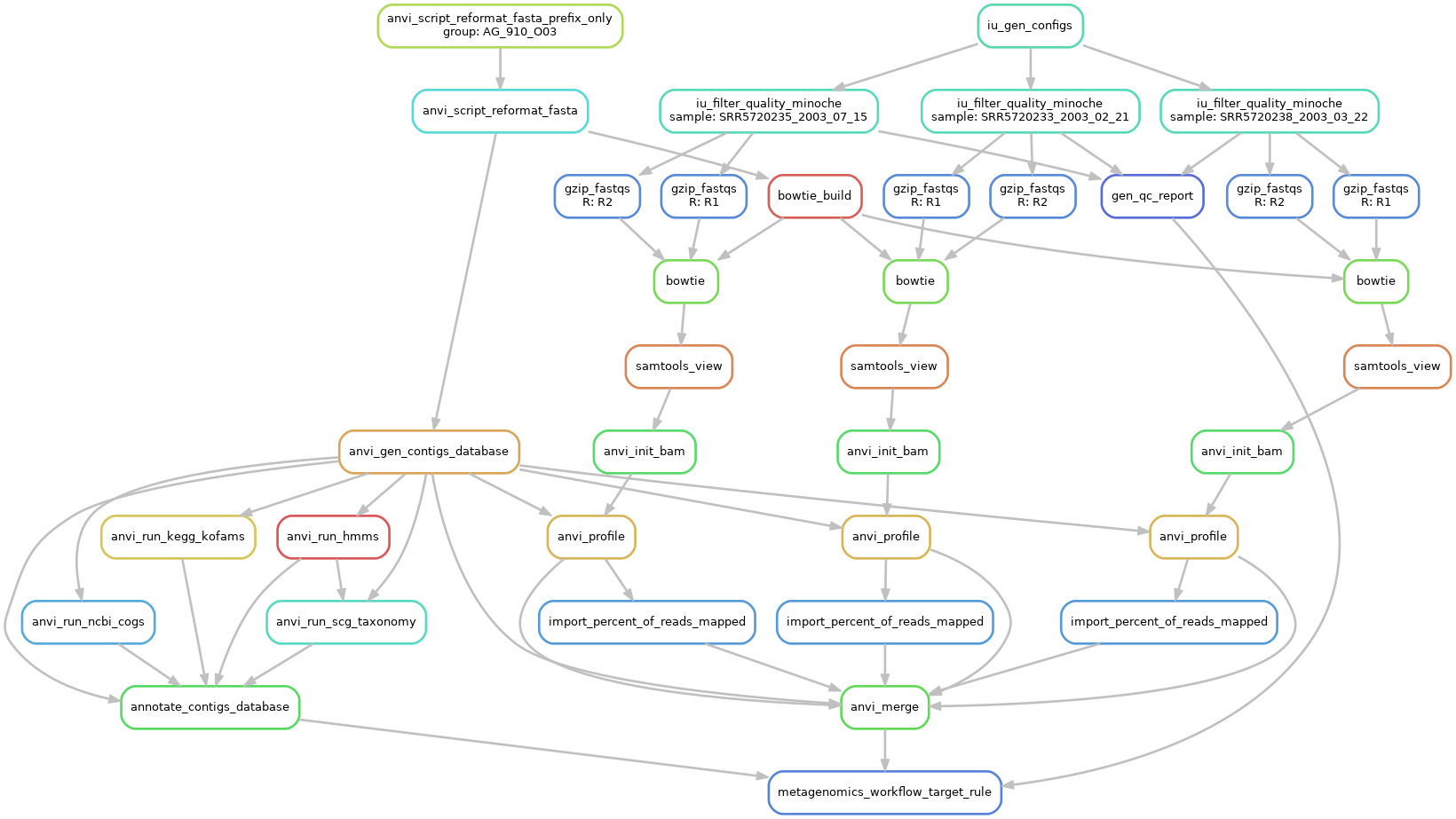
The interactive interface
First, let’s change to the right directory:
cd ../READ_RECRUITMENT
To start the interactive interface, you can use this command:
anvi-interactive -c CONTIGS/AG_910_O03-contigs.db -p PROFILE/PROFILE.db
If you click on the Draw button, you should see this:
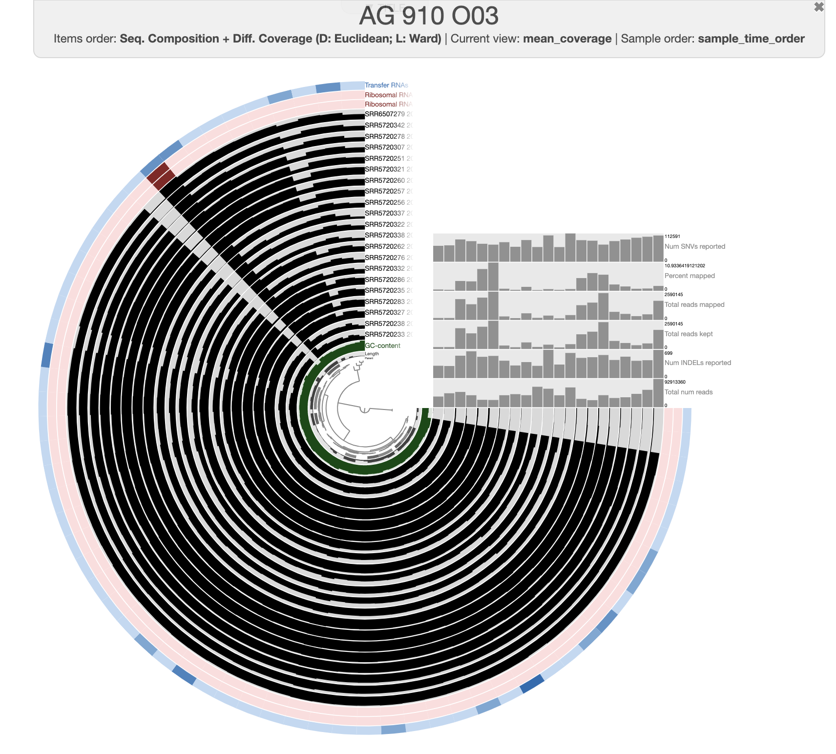
The central dendrogram represents contigs, or more precisely, ‘splits’ - as anvi’o splits large contigs into smaller (~20,000bp) sequences for a better visualization experience. Every layer represents a metagenome and the bar plot represents the mean coverage of a ‘split’ in a given metagenome.
By default the central dendrogram is computed using differential coverage and the sequence composition of the contigs (kmer composition, default k=4). You can also use only differential coverage, or only sequence composition with the View menu in the Main tab. Don’t forget to re-draw the figure to see the new contig organization.
You can polish the figure a little bit, especially by highlighting the percent of reads mapping to appreciate the seasonality pattern of Pelagibacter.
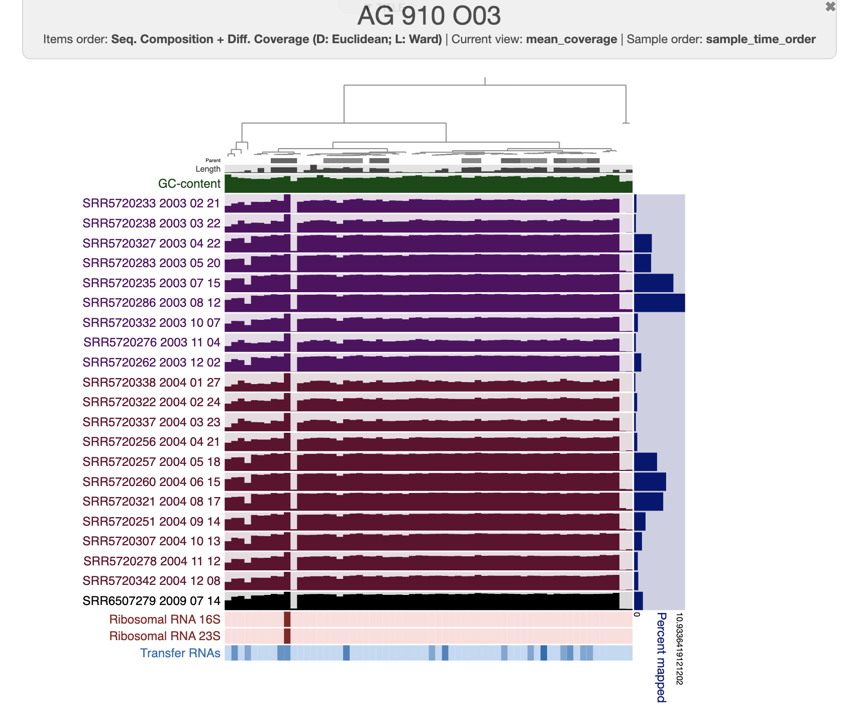
You probably immediately notice that three splits don’t have any coverage in all of the metagenomes! To check if it is contamination, you can select or ‘bin’ these splits with no coverage and open the Bin tab. You will see that these three splits only add up to ~42 kbp, nothing close to a full genome. You can also check for the presence of single-copy core genes present in these splits compared to the rest of the genome; you will see that there are none.
Another interesting observation is that one of the splits is actually part of a large contig containing an rRNA operon, so unless there is a misassembly, this split is definitely part of the genome.
The inspection page
To further investigate the content of splits, you can right click on one split and select Inspect split. It will open another tab on your browser with a more detailed view of the coverage. Using the Settings panel, you can choose to display SNVs and indels, overlay GC content, and color genes by their COG category or KEGG class.
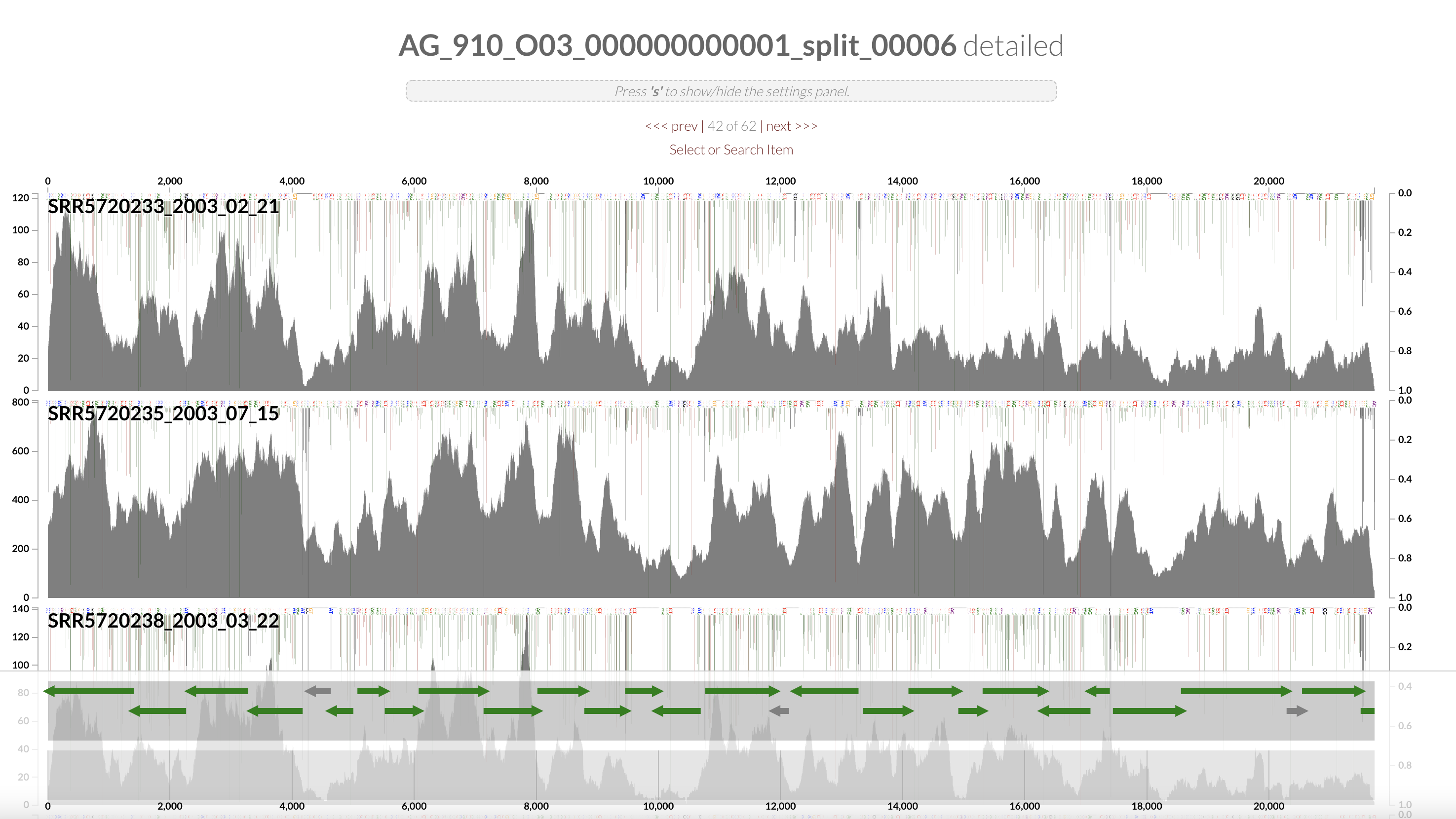
If you select a gene, you will see its functional annotation (if any) and you will be able to get its DNA and amino acid sequences. You can also directly start various BLAST jobs against NCBI nucleotide collection (nr) or the RefSeq genome database, using either blastn for the nucleotide sequence or blastx for the translated amino acid sequence.
Try inspecting the two splits with no coverage and have a look at the gene annotations (or lack thereof) to better understand why it is not detected in the environment. You will see that they contain genes associated with the cell wall and membrane!
Summarizing the read recruitment
Similar to the pangenomic analysis, we can summarize the results of the read recruitment using anvi-summarize. To summarize the whole SAG, you need to tell anvi’o that you want everything in that contigs db, not just a subset of contigs. To do that, we can create a ‘bin’ which contains all of the contigs. You could do it in the interactive interface and save it in a collection of your choice, or you can use the program anvi-script-add-default-collection:
anvi-script-add-default-collection -c CONTIGS/AG_910_O03-contigs.db -p PROFILE/PROFILE.db
And summarize the collection called ‘DEFAULT’ (or whatever name you gave it):
anvi-summarize -c CONTIGS/AG_910_O03-contigs.db \
               -p PROFILE/PROFILE.db \
               -C DEFAULT \
               -o SUMMARY
Here are all the files generated for this SAG (‘EVERYTHING’ is the default bin name created by anvi-script-add-default-collection; it could be different if you named your bin in the interactive interface):
$ ls SUMMARY/bin_by_bin/EVERYTHING/
EVERYTHING-Archaea_76-hmm-sequences.txt        EVERYTHING-Ribosomal_RNA_18S-hmm-hits.txt      EVERYTHING-Transfer_RNAs-hmm-sequences.txt     EVERYTHING-percent_completion.txt
EVERYTHING-Bacteria_71-hmm-sequences.txt       EVERYTHING-Ribosomal_RNA_18S-hmm-sequences.txt EVERYTHING-abundance.txt                       EVERYTHING-percent_redundancy.txt
EVERYTHING-GC_content.txt                      EVERYTHING-Ribosomal_RNA_23S-hmm-hits.txt      EVERYTHING-contigs.fa                          EVERYTHING-scg_domain.txt
EVERYTHING-N50.txt                             EVERYTHING-Ribosomal_RNA_23S-hmm-sequences.txt EVERYTHING-detection.txt                       EVERYTHING-scg_domain_confidence.txt
EVERYTHING-Protista_83-hmm-sequences.txt       EVERYTHING-Ribosomal_RNA_28S-hmm-hits.txt      EVERYTHING-gene_calls.txt                      EVERYTHING-scg_taxonomy_details.txt
EVERYTHING-Ribosomal_RNA_12S-hmm-hits.txt      EVERYTHING-Ribosomal_RNA_28S-hmm-sequences.txt EVERYTHING-mean_coverage.txt                   EVERYTHING-std_coverage.txt
EVERYTHING-Ribosomal_RNA_12S-hmm-sequences.txt EVERYTHING-Ribosomal_RNA_5S-hmm-hits.txt       EVERYTHING-mean_coverage_Q2Q3.txt              EVERYTHING-total_length.txt
EVERYTHING-Ribosomal_RNA_16S-hmm-hits.txt      EVERYTHING-Ribosomal_RNA_5S-hmm-sequences.txt  EVERYTHING-num_contigs.txt                     EVERYTHING-variability.txt
EVERYTHING-Ribosomal_RNA_16S-hmm-sequences.txt EVERYTHING-Transfer_RNAs-hmm-hits.txt          EVERYTHING-original_split_names.txt
If you were interested in only a part of the genome, like the contigs with no coverage, you can always bin these contigs to create a different collection and then summarize that collection. This would give you the contigs’ sequences, gene calls, functional annotations, and more.
In this example, we have only used one SAG for read recruitment. One of the drawbacks with this is the large amount of non-specific mapping (from different populations in the environment) to conserved genes/operons. You could recruit reads like this to every single SAG, one by one. But a better strategy to reduce non-specific mapping would be to concatenate all SAGs (or a subset of them) into a single FASTA file and map short-reads onto all of them at the same time. In that case, the read mapping would be competitive and you would be able to appreciate the variation of coverage between SAGs in the same sample. In order to reconcile which contigs in the contigs db belong to which SAG, you can import a collection listing all of the contigs and their associated SAG with anvi-import-collection.
Other anvi’o resources
Thanks for following this tutorial which shows you how to integrate single-cell genomics in anvi’o. There are many possible analysis that you can perform and we have just scratched the surface here. In the end, it is up to you to choose what you want to do with your data and what question you want to address.
There are many more tutorials and examples analysis with anvi’o and here is a list of some of them which could be relevant for your science:
- The infant gut tutorial is an all in one tutorial using a small set of metagenomes. I covers genome-resolved metagenomics, binning, phylogenomics, pangenomics, metabolism prediction, population genetics and protein structure variation.
- Studying microbial population genetics with anvi’o, an insight into SNVs, SCVs (codon) and SAAVs (amino acid) variation analysis.
- A simple read recruitment exercise.
- An exercise on metabolic reconstruction.
- A tutorial on the anvi’o interactive interface.
And more at https://anvio.org/#learn.