An anvi'o tutorial with Trichodesmium genomes (Chapter 2)


Table of Contents
About this page This webpage is one chapter of a much larger effort to cover multiple aspects of anvi’o in the same tutorial. If you need more context, please visit the main page of the tutorial, where you will find information about the dataset we are working with and the commands to download the tutorial datapack.
Quick Navigation
- Tutorial introduction (main page)
- Chapter 1: Genomics
- Chapter 2: Pangenomics ← you are here
- Chapter 3: Phylogenomics
- Chapter 4: Metabolism
Pangenomics
Show/Hide Starting the tutorial at this section? Click here for data preparation steps.
If you haven’t run previous sections of this tutorial (particularly the ‘Working with multiple genomes’ section), then you should follow these steps to setup the files that we will use going forward.
cp 00_DATA/contigs/*-contigs.db .
anvi-script-gen-genomes-file --input-dir . -o external-genomes.txt
anvi-estimate-scg-taxonomy -e external-genomes.txt -o taxonomy_multi_genomes.txt
Pangenomics represents a set of computational strategies to compare and study the relationship between a set of genomes through gene clusters. For a more comprehensive introduction into the subject, see this video.
Since the core concept of pangenomics is to compare genomes based on their gene content, it is important to know which genomes you plan you to use. Pangenomics is typically used with somewhat closely related organisms, at the species, genus, or sometimes family level. It is also valuable to check the estimated completeness and overall quality of the genomes you want to include in your pangenome analysis.
Low completeness genomes are likely missing some portion of their gene content. For that reason, we will include 7 out of the 8 Trichodesmium genomes to compute a pangenome. We won’t use the Trichodesmium thiebautii H9_4 because of its low estimated completeness and overall smaller genome size.
The inputs will be the contigs databases that are present in the datapack, plus the contigs-db of the Trichodesmium MAG that you downloaded in the first part of this tutorial.
$ ls 00_DATA/contigs
MAG_Candidatus_Trichodesmium_miru-contigs.db     MAG_Trichodesmium_thiebautii_Atlantic-contigs.db Trichodesmium_sp-contigs.db
MAG_Candidatus_Trichodesmium_nobis-contigs.db    MAG_Trichodesmium_thiebautii_Indian-contigs.db   Trichodesmium_thiebautii_H9_4-contigs.db
MAG_Trichodesmium_erythraeum-contigs.db          Trichodesmium_erythraeum_IMS101-contigs.db
Genome storage
The first step to compute a pangenome in anvi’o is the command anvi-gen-genomes-storage, which takes multiple contigs databases as input and generates a new anvi’o database called the genomes-storage-db. This database holds all gene information like functional annotations and amino acid sequences in a single location.
The input to anvi-gen-genomes-storage is an external-genomes file. You should have one from the previous tutorial section about working with multiple genomes (or from running the data preparation steps above). We just need to remove the Trichodesmium thiebautii H9_4:
grep -v Trichodesmium_thiebautii_H9_4 external-genomes.txt > external-genomes-pangenomics.txt
Then we can use the command anvi-gen-genomes-storage:
# make a directory of the pangenome analysis
mkdir -p 01_PANGENOME
anvi-gen-genomes-storage -e external-genomes-pangenomics.txt -o 01_PANGENOME/Trichodesmium-GENOMES.db
Pangenome analysis
To actually run the pangenomic analysis, we will use the command anvi-pan-genome. The sole input is the genomes-storage-db and it will generate a new database, called the pan-db:
# will take several minutes
anvi-pan-genome -g 01_PANGENOME/Trichodesmium-GENOMES.db \
                -o 01_PANGENOME \
                -n Trichodesmium \
                -T 4
Under the hood, anvi-pan-genome uses DIAMOND (or BLASTp if you choose the alternative) to compute the similarity between amino acid sequences from every genomes. From this all-vs-all search, it will use the MCL algorithm to cluster the genes into groups of relatively high similarity. The pan-db stores the gene cluster information.
Interactive pangenomics display
Now that we have a genomes-storage-db and a pan-db, we can use the command anvi-display-pan to start an interactive interface of our pangenome:
anvi-display-pan -g 01_PANGENOME/Trichodesmium-GENOMES.db -p 01_PANGENOME/Trichodesmium-PAN.db
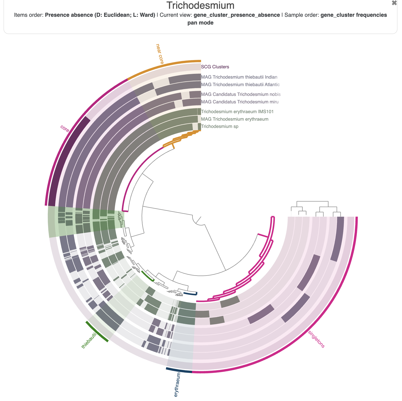
And here is what you should see in your browser:
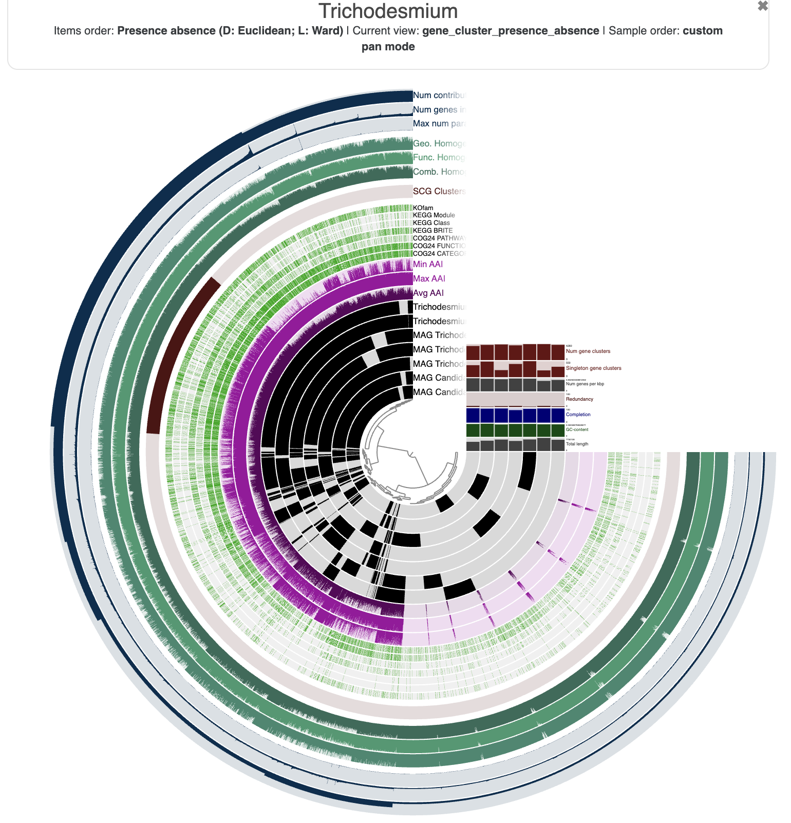
You are seeing:
- The genomes in black layers.
- The inner dendrogram: every leaf of that dendrogram is a gene cluster.
- The black heatmap: presence/absence of a gene from a genome in a gene cluster.
- Multiple colorful additional layers with information about the underlying gene cluster.
- Some layer (genome) data at the right-end of the circular heatmap.
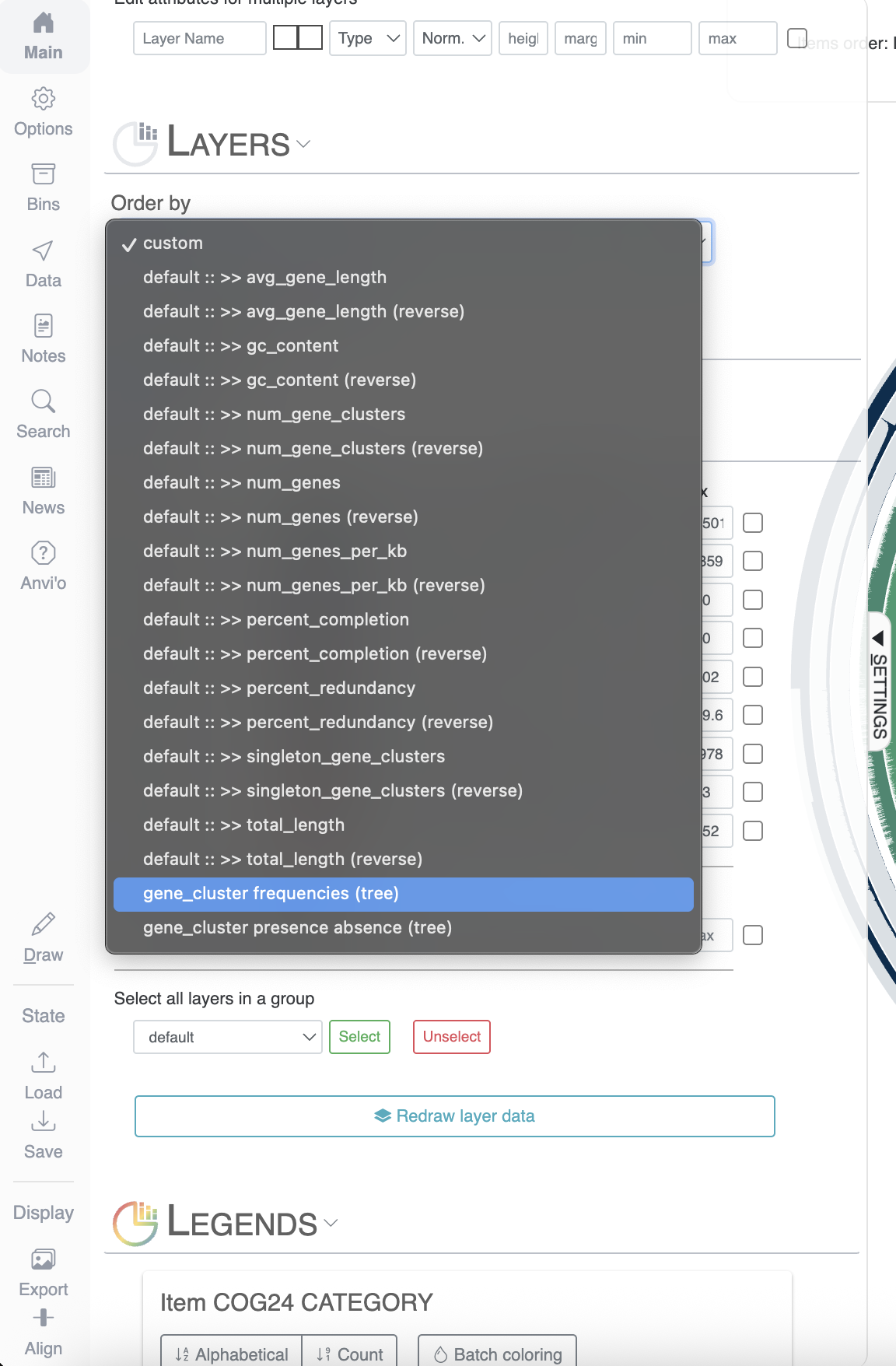
First of all, let’s reorder the genomes. By default they will simply appear in alphabetical order, which is not very interesting. In the main panel, you can scroll down to “Layers” and select gene_cluster_frequency:
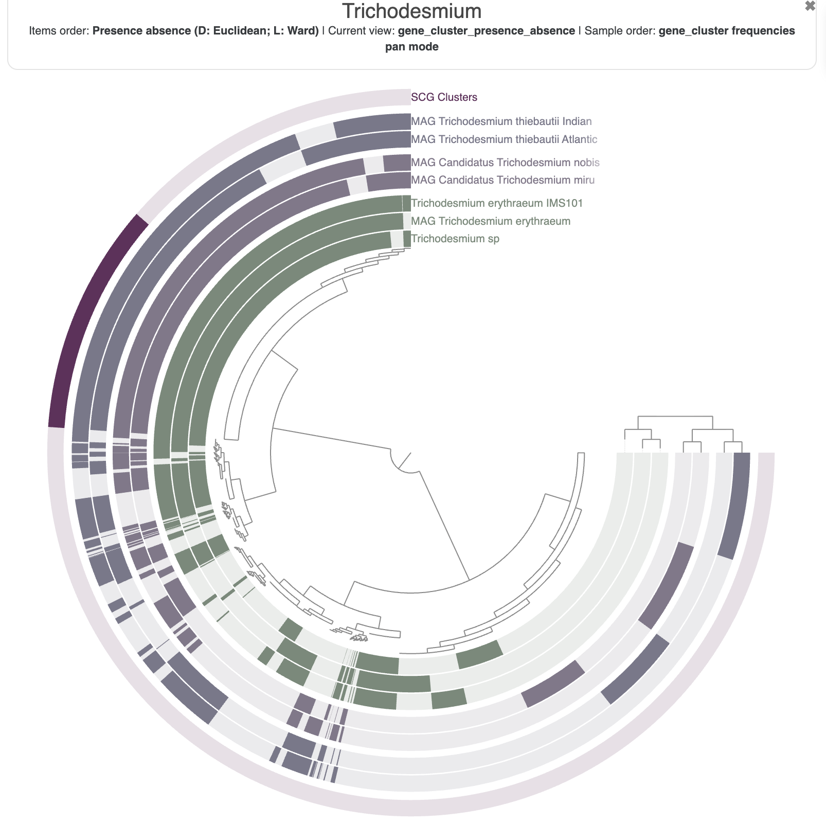
The resulting figure will now pull together genomes that share similar gene content. It may not be very noticeable at first but if you pay attention between the before/after you will notice that we have now two clusters (see dendrogram on the right):
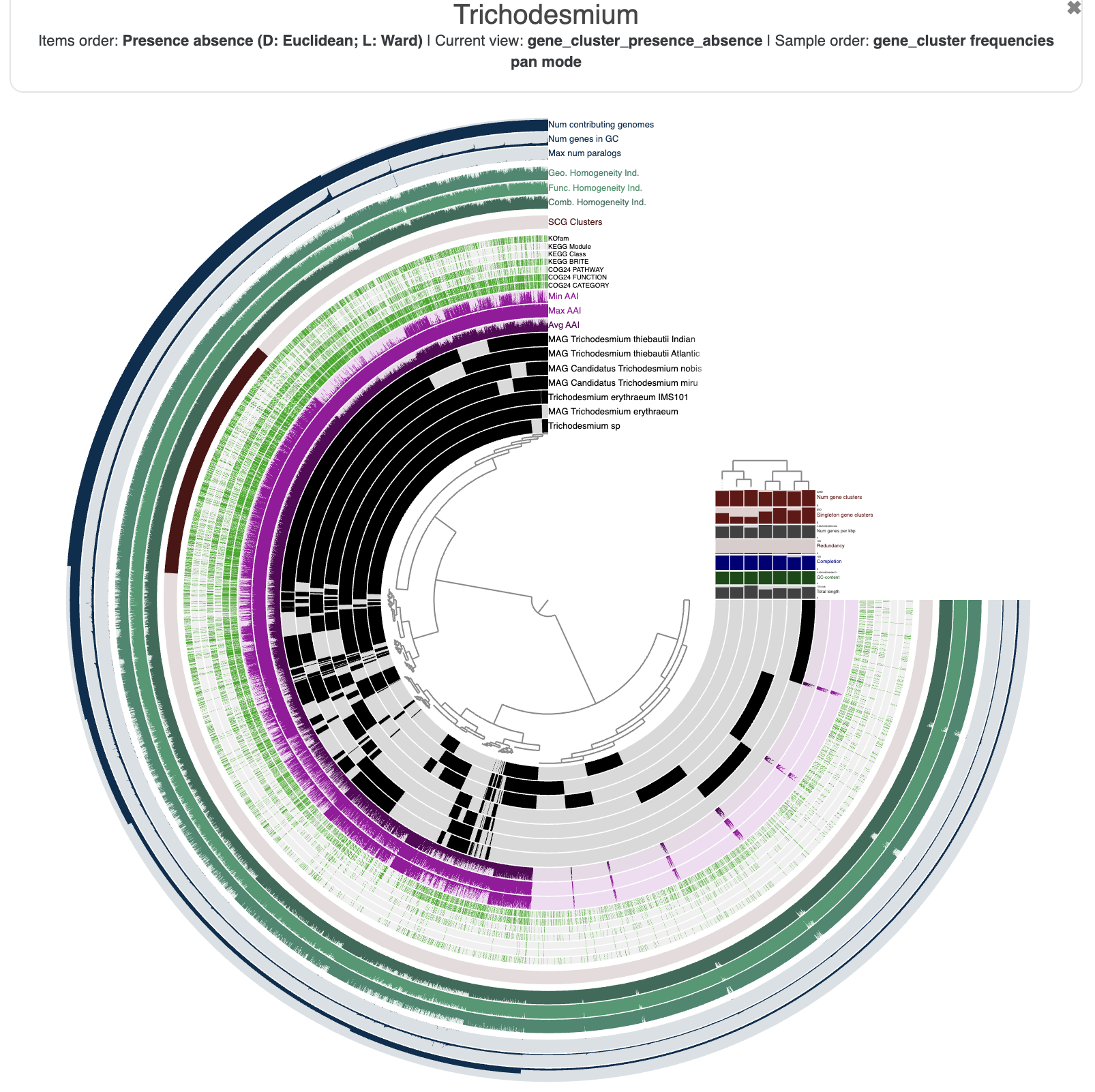
This figure was made with a dendrogram radius of 4500. You can change the radius in the Options tab.
Now that you have made some modifications to your interactive figure, it would be a good idea to save those settings. The aesthetics of a figure are saved in a “state”, and you will find a button on the bottom left of the interface to save it. You can store multiple states for the same pangenome (different colors, different layers being displayed, etc). The state called default will always be the one displayed when you start an interactive interface. The state can also be exported/imported from the terminal with the programs anvi-export-state and anvi-import-state.
You can spend some time getting familiar with the interface and all the possible customisation options. For instance, here is the pangenome figure I made:
The state to reproduce the figure above is available in the directory 00_DATA, and you can import it with the following command:
anvi-import-state -p 01_PANGENOME/Trichodesmium-PAN.db -s 00_DATA/pan_state.json -n tutorial_state
Inspect gene clusters
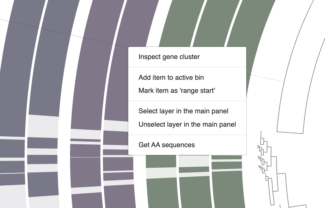
Every gene cluster contains one or more amino acid sequences from one or more genomes. In some cases, they may contain multiple genes from a single genome (i.e., multi-copy genes). You can use your mouse and select a gene cluster on the interface, right-click and select Inspect gene cluster:
It will open a new tab with the multisequence alignment of the amino acid sequences in the cluster:
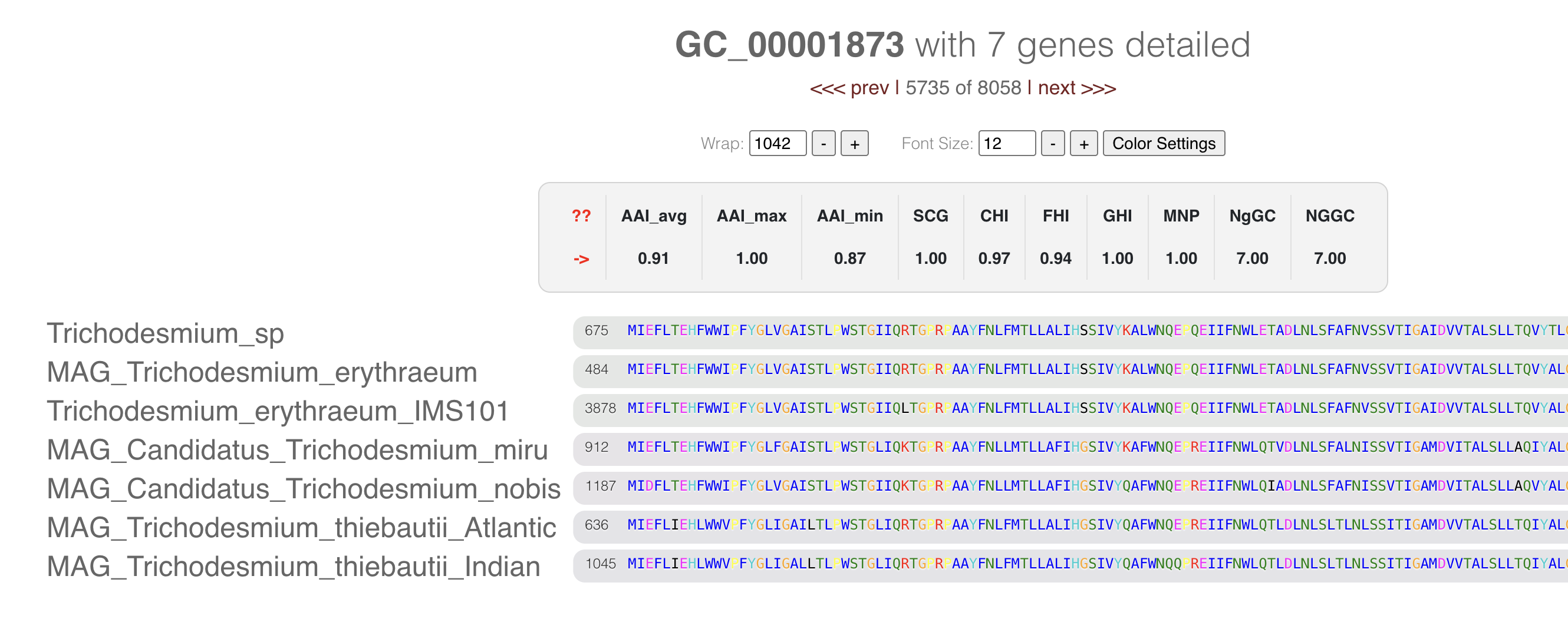
If you want to know more about the amino acid coloring, you can check this blog post by Mahmoud Yousef. In brief, the colors represent the amino acid properties (like polar, cyclic) and their conservancy in the alignment.
If you click on one of the gene caller ID numbers you will get some information about that gene:
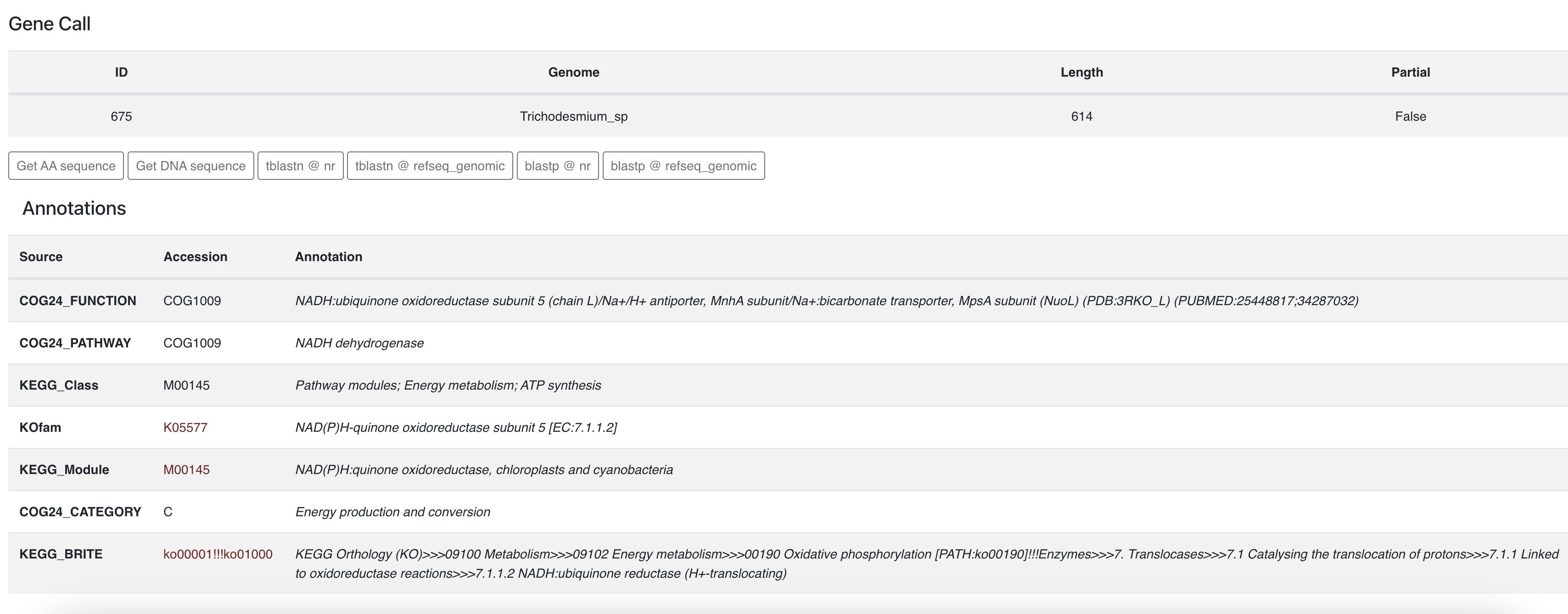
From there you can learn about its functional annotations, if any. You can also retrieve the amino acid sequence and start some BLAST commands on the NCBI servers.
Bin and summarize a pangenome
Looking at individual genes clusters is great, but not very practical to summarize a large selection of gene clusters. Fortunately for you, you can select gene clusters in the main interface and create ‘bins’ which you can meaningfully rename. In the next screenshot, I have selected the core genome, the near core, the accessory genome of Trichodesmium erythraeum and Trichodesmium thiebautii, and all the singleton gene clusters.
Once you are happy with your bins, don’t forget to save them into a collection. Just like the ‘state’ saves the current settings for the figure, the ‘collection’ stores your selection of items, here gene clusters. You can save as many collections as you want, and the collection called default will always appear when you start the interactive interface with anvi-display-pan.
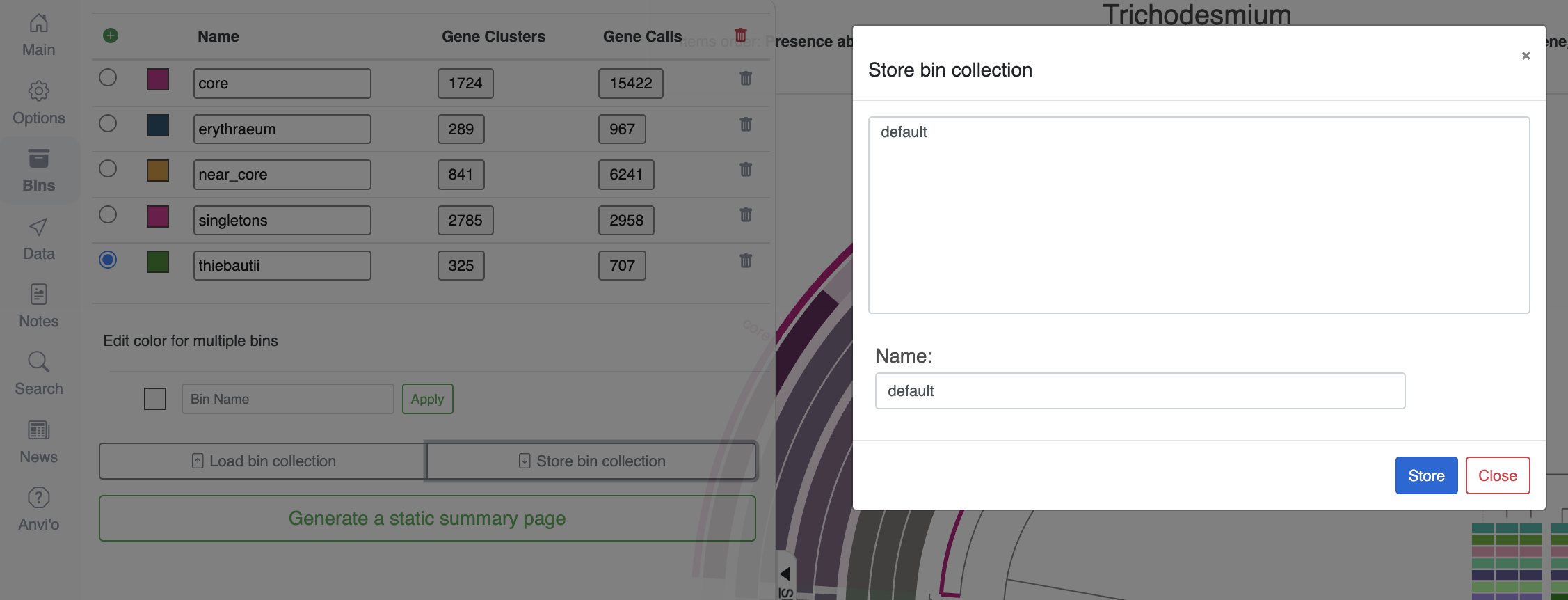
Now that we have some meaningful bins, it is time to make sense of their content by either using the program anvi-summarize, or selecting Generate a static summary page in the “Bins” tab of the interface.
Here is how you would do it with the command line (note that I named my collection “default”):
anvi-summarize -g 01_PANGENOME/Trichodesmium-GENOMES.db \
               -p 01_PANGENOME/Trichodesmium-PAN.db \
               -C default \
               -o 01_PANGENOME/SUMMARY
The interactive interface button and the above command generate the same output directory, which contains a large table summarizing ALL genes from all genomes. Here are the first few rows:
unique_id |
gene_cluster_id |
bin_name |
genome_name |
gene_callers_id |
num_genomes_gene_cluster_has_hits |
num_genes_in_gene_cluster |
max_num_paralogs |
SCG |
functional_homogeneity_index |
geometric_homogeneity_index |
combined_homogeneity_index |
AAI_min |
AAI_max |
AAI_avg |
COG24_PATHWAY_ACC |
COG24_PATHWAY |
COG24_FUNCTION_ACC |
COG24_FUNCTION |
KEGG_BRITE_ACC |
KEGG_BRITE |
KOfam_ACC |
KOfam |
COG24_CATEGORY_ACC |
COG24_CATEGORY |
KEGG_Class_ACC |
KEGG_Class |
KEGG_Module_ACC |
KEGG_Module |
aa_sequence |
|---|---|---|---|---|---|---|---|---|---|---|---|---|---|---|---|---|---|---|---|---|---|---|---|---|---|---|---|---|---|
| 1 | GC_00000001 | near_core | MAG_Candidatus_Trichodesmium_miru | 3624 | 6 | 221 | 214 | 0 | 0.659555877418382 | 0.940765773081969 | 0.775453602988201 | 0.12124248496994 | 1.0 | 0.956257104913241 | ——————————————————————————————————————————————————————————————————————————————————————————————————————————————————————————————————————————————————MQSWAAEELKYTNLPDKRLNQRLIKIVEQASAQPEASVPQASGDWANTKATYYFWNSERFSSEDIIDGHRRSTAQRASQEDVILAIQDTSDFNFTHHKGKTWDKGFGQTCSQKYVRGLKVHSTLAVSSQGVPLGILDLQIWTREPNKKRKKKKSKGSTSIFNKESKRWLRGLVDAELAIPSTTKIVTIADREGDMYELFALVILANSELLIRANHNRRVNHEMKYLRDRFSQAPEAGKLKVSVPKKDGQPLREATLSIRYGMLTICAPNNLSQGNNRSPITLNVISAVEENFAEGVKPINWLLLTTKEVDNFEDAVGCIRWYTYRWLIERYHYVLKSGCGIEKLQLKTAQRIKKALATYALVAWRLLWLTYHGRENPQLKSDKVLEQHEWQSLYCHFHCTSIAPAQPPSLKQAMVWIAKLGGFLGRKNDGEPGVKSLWRGLKRLHDIASTWKLAHSSTSIACESYR———————————————————————————————- | ||||||||||||||
| 2 | GC_00000001 | near_core | MAG_Candidatus_Trichodesmium_nobis | 940 | 6 | 221 | 214 | 0 | 0.659555877418382 | 0.940765773081969 | 0.775453602988201 | 0.12124248496994 | 1.0 | 0.956257104913241 | ——————————————————————————————————————————————————————————————————————————————————————————————————————————————————————————————————————————————————MQSWAAEELKYTNLPDKRLNQRLIKIVEQASAQPEASVPQASGDWANTKATYYFWNSERFSSEDIIDGHRRSTAQRASQEDVILAIQDTSDFNFTHHKGKTWDKGFGQTCSQKYVRGLKVHSTLAVSSQGVPLGILDLQIWTREPNKKRKKKKSKGSTSIFNKESKRWLRGLVDAELAIPSTTKIVTIADREGDMYELFALVILANSELLIRANHNRRVNHEMKYLRESISQAPEAGKLKVSVPKKDGQPLREATLSIRYGMLTISASNNLSQGNNRSPITLNVIYAVEENFAEGVKPINWLLLTTKEVDNFEDAVGCIRWYTYRWLIERYHYVLKSGCGIEKLQLETAQRIKKALATYALVAWRLLWLTYHGRENPQLKSDTVLEQHEWQSLYCHFHCTSIAPAQPPSLKQAMVWIAKLGGFLGRKNDGEPGVKSLWRGLKRLHDIASTWKLAHSSTSIACESYG———————————————————————————————- | ||||||||||||||
| 3 | GC_00000001 | near_core | MAG_Candidatus_Trichodesmium_nobis | 682 | 6 | 221 | 214 | 0 | 0.659555877418382 | 0.940765773081969 | 0.775453602988201 | 0.12124248496994 | 1.0 | 0.956257104913241 | ———————————————————————————————————————————————————————————————————————————————————————————————————————————————————————————————————————————MVWIAKLGGFLGSKNDGEPGVKSLW————————————————————————————————————————————————————————————————————————————————————————————————————————————————————————————————————————————————–RVLERLYDIASTWKLIHSSTSIACESYG———————————————————————————————- | ||||||||||||||
| 4 | GC_00000001 | near_core | MAG_Trichodesmium_erythraeum | 90 | 6 | 221 | 214 | 0 | 0.659555877418382 | 0.940765773081969 | 0.775453602988201 | 0.12124248496994 | 1.0 | 0.956257104913241 | ——————————————————————————————————————————————————————————————————————————————————————————————————————————————————————————————————————————–AMVWIAKLGGFLGRKNDGEPGVKSLW————————————————————————————————————————————————————————————————————————————————————————————————————————————————————————————————————————————————–RGLKRLHDIASTWKLAHSFTSIACESYG———————————————————————————————- | ||||||||||||||
| 5 | GC_00000001 | near_core | MAG_Trichodesmium_erythraeum | 143 | 6 | 221 | 214 | 0 | 0.659555877418382 | 0.940765773081969 | 0.775453602988201 | 0.12124248496994 | 1.0 | 0.956257104913241 | ——————————————————————————————————————————————————————————————————————————————————————————————————————————————————————————————————————————–AMVWIAKLGGFLGRKNDGEPGVKSLW————————————————————————————————————————————————————————————————————————————————————————————————————————————————————————————————————————————————–RGLKRLHDIASTWKLAHSFTSIACESYG———————————————————————————————- | ||||||||||||||
| 6 | GC_00000001 | near_core | MAG_Trichodesmium_erythraeum | 334 | 6 | 221 | 214 | 0 | 0.659555877418382 | 0.940765773081969 | 0.775453602988201 | 0.12124248496994 | 1.0 | 0.956257104913241 | ——————————————————————————————————————————————————————————————————————————————————————————————————————————————————————————————————————————–AMVWIAKLGGFLGRKNDGEPGVKSLW————————————————————————————————————————————————————————————————————————————————————————————————————————————————————————————————————————————————–RGLKRLHDIASTWKLAHSFTSIACESYG———————————————————————————————- | ||||||||||||||
| 7 | GC_00000001 | near_core | MAG_Trichodesmium_erythraeum | 601 | 6 | 221 | 214 | 0 | 0.659555877418382 | 0.940765773081969 | 0.775453602988201 | 0.12124248496994 | 1.0 | 0.956257104913241 | ——————————————————————————————————————————————————————————————————————————————————————————————————————————————————————————————————————————–AMVWIAKLGGFLGRKNDGEPGVKSLW————————————————————————————————————————————————————————————————————————————————————————————————————————————————————————————————————————————————–RGLKRLHDIASTWKLAHSFTSIACESYG———————————————————————————————- | ||||||||||||||
| 8 | GC_00000001 | near_core | MAG_Trichodesmium_erythraeum | 901 | 6 | 221 | 214 | 0 | 0.659555877418382 | 0.940765773081969 | 0.775453602988201 | 0.12124248496994 | 1.0 | 0.956257104913241 | ——————————————————————————————————————————————————————————————————————————————————————————————————————————————————————————————————————————–AMVWIAKLGGFLGRKNDGEPGVKSLW————————————————————————————————————————————————————————————————————————————————————————————————————————————————————————————————————————————————–RGLKRLHDIASTWKLAHSFTSIACESYG———————————————————————————————- | ||||||||||||||
| 9 | GC_00000001 | near_core | MAG_Trichodesmium_erythraeum | 917 | 6 | 221 | 214 | 0 | 0.659555877418382 | 0.940765773081969 | 0.775453602988201 | 0.12124248496994 | 1.0 | 0.956257104913241 | ——————————————————————————————————————————————————————————————————————————————————————————————————————————————————————————————————————————–AMVWIAKLGGFLGRKNDGEPGVKSLW————————————————————————————————————————————————————————————————————————————————————————————————————————————————————————————————————————————————–RGLKRLHDIASTWKLAHSFTSIACESYG———————————————————————————————- |
Search for functional annotations
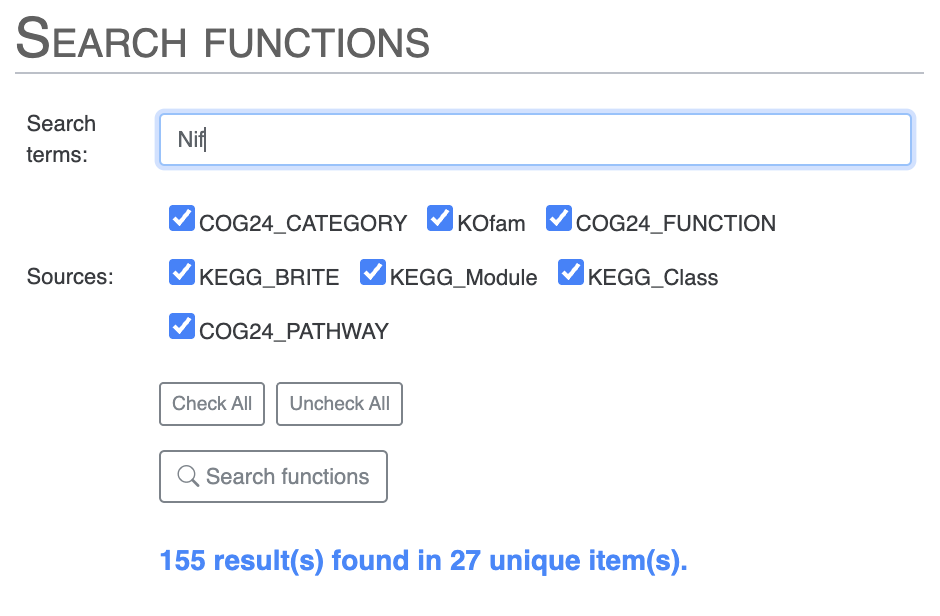
If you are interested in one or more functional annotations and where they fit in the pangenome - core, accessory, singleton, single or multiple copies - then you can use the “Search” tab. There you can search using any term you like. You can search for Nif and you will get all Nif genes, including NifH and more.
Or, you can directly search for NifH and you will notice two results which are not expected. As you might recall from the previous tutorial chapter, we know from Tom’s paper that COG mis-annotates a ferredoxin gene as NifH:
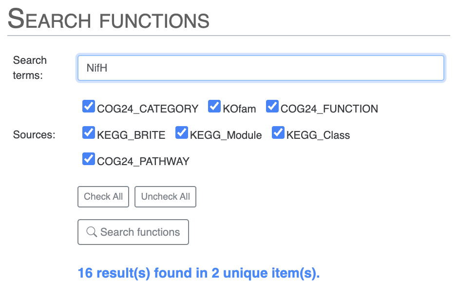
For instance, we found that genes with COG20 function incorrectly annotated as “Nitrogenase ATPase subunit NifH/coenzyme F430 biosynthesis subunit CfbC” correspond, in reality, to “ferredoxin: protochlorophyllide reductase.”
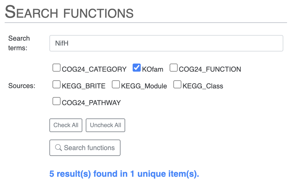
To avoid seeing the COG results, you can search for NifH by selecting only the KOfam annotation source, or directly use the KOfam accession number K02588:
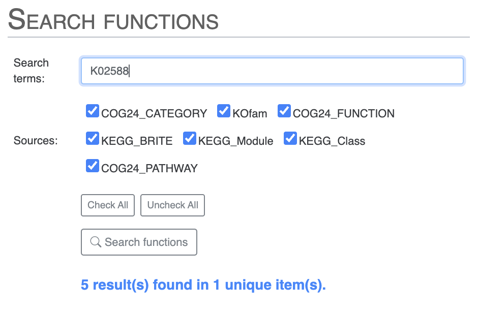
Then you can scroll down to where you can list the results of the search or choose to highlight them on the pangenome. I would suggest you look for all the Nif genes, using only the KOfam annotation source to avoid the issues with COG. Then highlight the results on your pangenome. You can even choose to add the search result items to a bin.
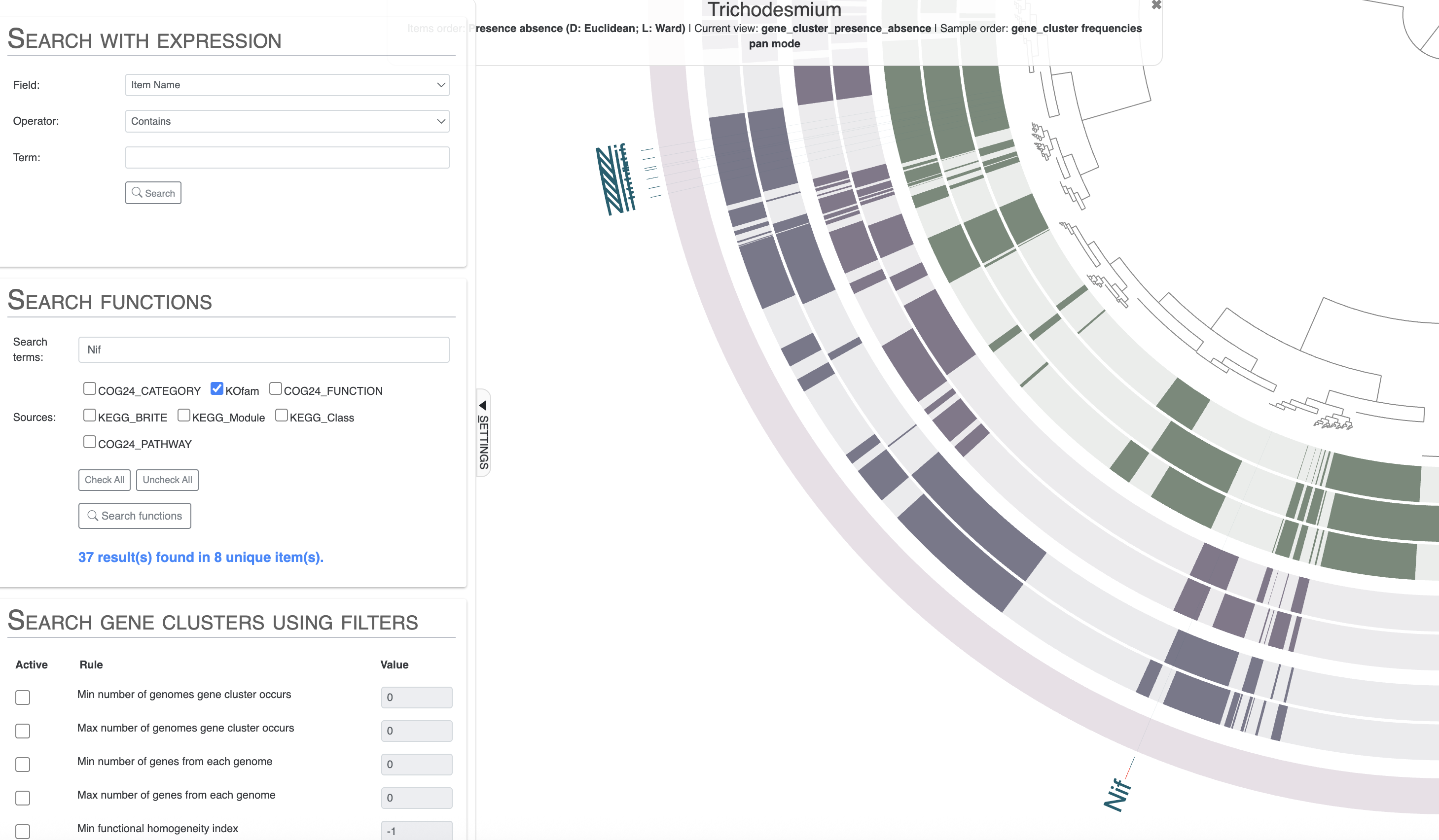
Note how nearly all Nif genes are concentrated in a section of the pangenome which correspond to gene clusters shared between Trichodesmium thiebautii and erythraeum, and not in Trichodesmium miru or nobis. The result is coherent with these genomes lacking nitrogen fixation capabilities, but you may be wondering what is happening for that single gene cluster on the lower part of the pangenome. It is found in T. miru, T. nobis and one T. thiebautii. If you inspect that gene cluster and look for the full functional annotation, you will see that it is NifU, which is not a marker for nitrogen fixation as it can be found in non-diazotrophic organisms.
Additional genome information
To help make sense of your pangenome, you can add multiple additional data layers with information about the genomes you are using. We will see how you can add the taxonomy information that we computed earlier, and also the pairwise average nucleotide identity of these genomes.
Add taxonomy
We previously (this section in Chapter 1) used anvi-estimate-scg-taxonomy and made a text output called taxonomy_multi_genomes.txt. We can import that table directly into the pangenome with the command anvi-import-misc-data:
anvi-import-misc-data -p 01_PANGENOME/Trichodesmium-PAN.db \
                      -t layers \
                      --just-do-it \
                      taxonomy_multi_genomes.txt
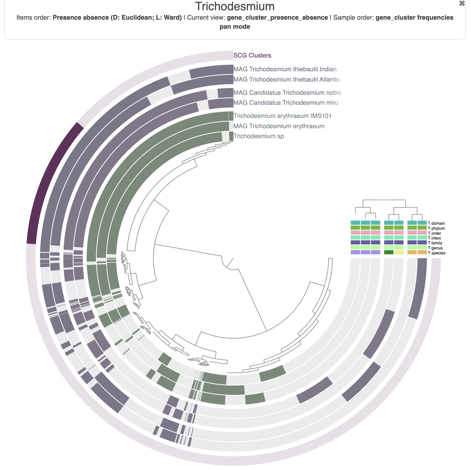
Nothing very surprising, but it is always good to see that the taxonomy agrees with how the genomes are currently organized, i.e. by their gene content.
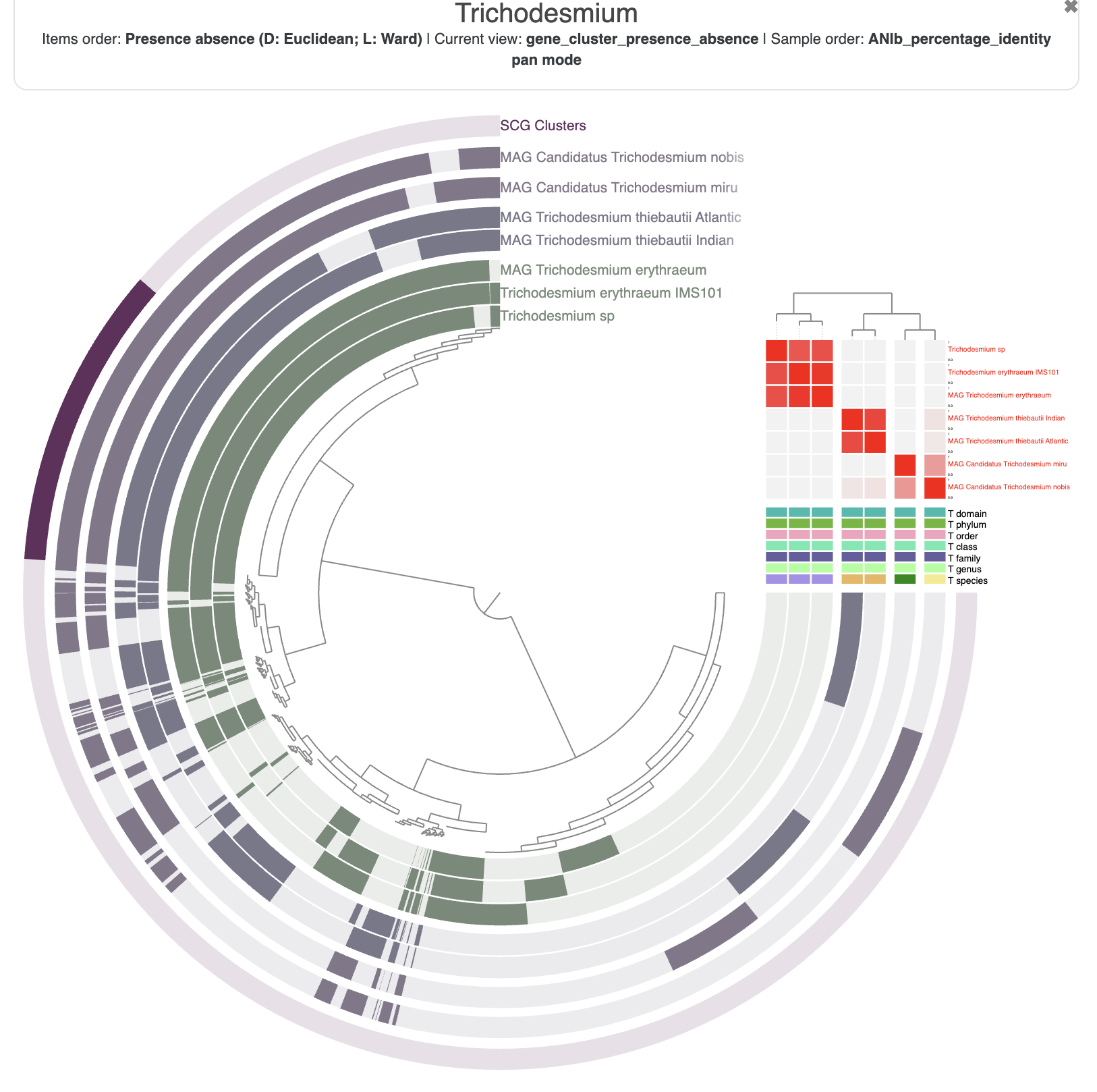
Compute average nucleotide identity
A companion metric to pangenomes is the Average Nucleotide Identity, or ANI, which is based on whole genome DNA similarity. There is a program called anvi-compute-genome-similarity that allows you to use your contigs-db and three different methods to compute ANI. By default it uses PyANI, but you can also choose FastANI.
The sole required input is an external-genomes file, and the output is a directory with multiple files containing the ANI value, coverage, and more. Optionally, you can also provide a pan-db and anvi’o will import the ANI values directly into your pangenome.
## takes ~9 minutes
anvi-compute-genome-similarity -e external-genomes-pangenomics.txt \
                               -p 01_PANGENOME/Trichodesmium-PAN.db \
                               -o 01_PANGENOME/ANI \
                               --program pyANI \
                               -T 4
You should check the content of the output directory, 01_PANGENOME/ANI. It contains multiple matrices and associated tree files.
A friendly reminder that the ANI is computed on the fraction of two genomes that align to each other. Any genomic segment that is not found in one of the genomes is not taken into account in the final percent identity. The output of PyANI includes the alignment coverage of the pairwise genome comparison, and also the full_percentage_identity which correspond to ANI * coverage. Also note that ANI is not a symmetrical value.
When you start the interactive interface with anvi-display-pan, you should be able to select the ANI identity values in the layer section of the main panel. You can also reorder the genomes based on the ANI similarities in the “layers” section of the main table.
Integrating ecology and evolution with metapangenomes
AS you can see from the example above, you can integrate a lot of information in a single anvi’o figure. And not just the figure, as the pan-db contains all the information in the interactive display as well.
Another topic not covered yet in this tutorial is metagenomic read recruitment, which allows you to compute detection and coverage of one or more genomes across metagenomes. This gives you an ecological signal and nothing is stopping you from importing a relative abundance heatmap, just like the ANI. There is a dedicated program for this in anvi’o, called anvi-meta-pan-genome, which you can learn more about here.
At the end of the day, you can have a figure like this one, with ecology and evolution integrated in one figure:
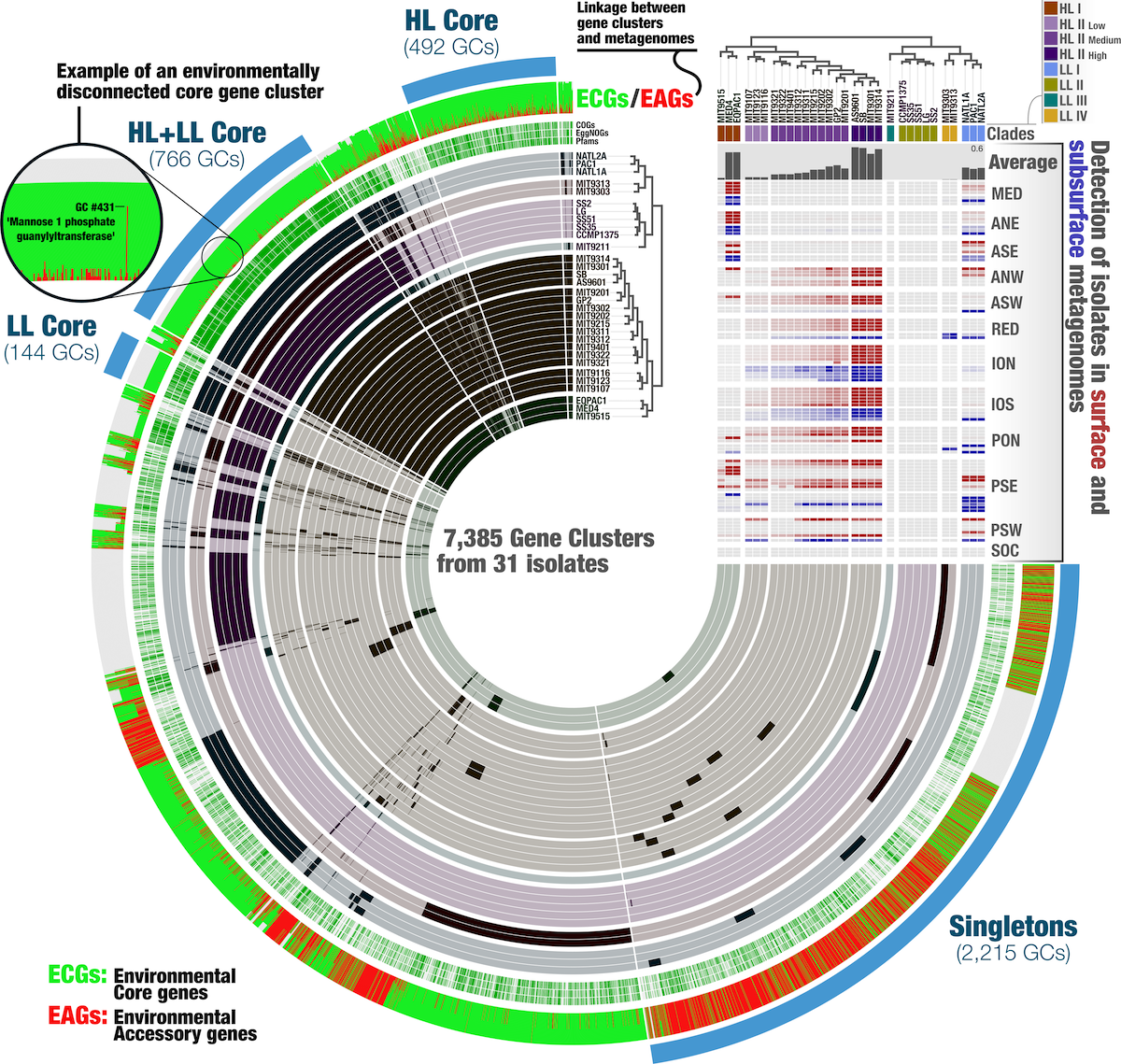
But that analysis is for another time.
The next chapter
If you want to immediately move on to the next chapter of this tutorial, here is the link:
If you want to go back to the main page of the tutorial instead, click here.
If you have any questions about this exercise, or have ideas to make it better, please feel free to get in touch with the anvi’o community through our Discord server: