An anvi'o tutorial with Trichodesmium genomes (Chapter 3)


Table of Contents
- Quick Navigation
- Chapter 3: Phylogenomics
- Placing Trichodesmium in evolutionary context
- Making a genomes file for phylogenomics
- Selecting genes for making the tree
- Getting a concatenated alignment
- Making an initial tree with FastTree
- Making another tree with IQ-Tree
- Adding misc data to the tree
- The next chapter
About this page This webpage is one chapter of a much larger effort to cover multiple aspects of anvi’o in the same tutorial. If you need more context, please visit the main page of the tutorial, where you will find information about the dataset we are working with and the commands to download the tutorial datapack.
Quick Navigation
- Tutorial introduction (main page)
- Chapter 1: Genomics
- Chapter 2: Pangenomics
- Chapter 3: Phylogenomics ← you are here
- Chapter 4: Metabolism
Chapter 3: Phylogenomics
Show/Hide Starting the tutorial at this section? Click here for data preparation steps.
If you haven’t run previous sections of this tutorial, then you should follow these steps to setup the files that we will use going forward.
cp 00_DATA/contigs/*-contigs.db .
anvi-script-gen-genomes-file --input-dir . -o external-genomes.txt
grep -v Trichodesmium_thiebautii_H9_4 external-genomes.txt > external-genomes-pangenomics.txt
If you want to understand the evolutionary relationships between microbes, phylogenomics is the tool for you. Phylogenomics is extremely similar to phylogenetics – they both compare sequences of the same gene coming from distinct genomes to estimate how those sequences are related, typically visualized as a tree. The only difference is that phylogenetics compares only a single gene (often 16S rRNA), while phylogenomics compares multiple genes. This larger basis for comparison often gives phylogenomic trees a higher resolution and accuracy – provided you are using the right genes.
What are the ‘right genes’? To capture an evolutionary signal, the genes you use for phylogenomics need to fulfill the following requirements:
- (1) they should be present in all of your genomes of interest
- (2) they should be in single-copy (no paralogs) so that there is only one version of each gene from each genome to compare
- (3) their sequences should be similar enough across genomes for good alignments, yet distinct enough to meaningfully capture evolutionary distances (this is what makes the 16S rRNA gene, with its variable regions, so valuable for phylogenies)
- (4) they shouldn’t be genes that undergo horizontal gene transfer, or HGT (to avoid confounding the evolutionary signal from vertical inheritance with the HGT signal)
Requirements (1) and (2) mean that single-copy core genes (SCGs) are good candidates for phylogenomics. However, not all SCGs fulfill requirements (3) and (4) – ensuring those are fulfilled may take some extra investigation. We often use ribosomal proteins (RPs) for phylogenomics because they tend to meet all the criteria. Of course, depending on your research question, you can make exceptions for some of these requirements; however, they are generally a good starting point for evolutionary investigations.
If you have created a pangenome from your genomes of interest, you can use it to filter for genes that could be useful for phylogenomics – either by searching within the anvi-display-pan interface, by generating a summary table with anvi-summarize, or by using the program anvi-get-sequences-for-gene-clusters. For instance, you can require gene clusters to occur in all genomes to fulfill (1), require a maximum of one gene from each genome in a given cluster to fulfill (2), and search for clusters with a low functional homogeneity index and a high geometric homogeneity index to fulfill (3). The only requirement the pangenomics doesn’t help you with is (4) – so you need to be somewhat cautious when using this method and make sure you aren’t inadvertently including genes prone to HGT.
Placing Trichodesmium in evolutionary context
We learned in the pangenomics chapter that our candidate Trichodesmium genomes form their own little group when clustered according to functional similarity. But how do these genomes fit in with the other Trichodesmium species when we consider their evolutionary relationships? We will use phylogenomics to answer this question.
But looking at only the Trichodesmium genomes out of context could be a bit boring. So let’s make it just a little bit more interesting by adding a few other well-known cyanobacteria so that we can see how Trichodesmium relates to those genomes. We will work with the following additional cyanobacteria:
- Prochlorococcus marinus (one of the most abundant photosynthetic organisms around the globe),
- its closely-related friend Synechococcus elongatus, and
- another well-known candidate species that is an obligate symbiont of algae, Ca. Atelocyanobacterium thalassa (also known as UCYN-A, for ‘unicellular cyanobacterial group A’).
If you are a marine microbiologist, you will probably know all those names and how they relate to each other very well, so there will be no further surprises for you in this tutorial. But if not, now is your chance to learn how to place the “big names” of marine microbial photosynthesis onto a tree. :)
There is just one more thing missing. In order to study the evolutionary relationships between all these cyanobacteria, we need an ‘outgroup’ – a microbe that we know is not a cyanobacteria and that we can place at the ‘root’ of the tree to serve as a reference point of comparison. For our purposes today, which outgroup bacteria we use doesn’t matter very much, so just for fun, we are going to use yet another “big name” microbe from the marine environment: Ca. Pelagibacter ubique (also known as SAR11), the most abundant life form in the ocean.
All four of these additional genomes are already available in the datapack as contigs databases:
$ ls 00_DATA/phylo_dbs/
GCF_000012345-contigs.db GCF_000015665-contigs.db GCF_000025125-contigs.db GCF_022984195-contigs.db
They have been annotated in the same way as the Trichodesmium genomes, including with anvi-run-hmms so that we have the annotations for single-copy core genes available.
Making a genomes file for phylogenomics
To keep things organized, let’s make a directory in which to store all our trees and associated files:
mkdir 02_PHYLOGENOMICS
We’re going to combine the 7 Trichodesmium genomes that we used for pangenomics (skipping the incomplete MAG, Trichodesmium thiebautii H9_4) with the 4 additional marine bacteria. To do so, we first use anvi-script-gen-genomes-file to make an external-genomes file including the four new contigs databases, and then we concatenate that file (minus its header line) with our previous external-genomes file from the pangenomics analysis:
anvi-script-gen-genomes-file --input-dir 00_DATA/phylo_dbs/ -o 02_PHYLOGENOMICS/cyano-genomes.txt

# combine into one external genomes file
cat external-genomes-pangenomics.txt <(tail -n+2 02_PHYLOGENOMICS/cyano-genomes.txt) > 02_PHYLOGENOMICS/external-genomes-phylogenomics.txt
Selecting genes for making the tree
The next step is to figure out which bacterial single-copy core genes we want to use to make the phylogenomic tree. The program anvi-get-sequences-for-hmm-hits will help us extract those gene sequences, and it conveniently has an -L (or --list-available-gene-names) option that allows us to preview which genes are available in each collection of SCGs:
anvi-get-sequences-for-hmm-hits -e 02_PHYLOGENOMICS/external-genomes-phylogenomics.txt -L
In the resulting terminal output, you should see the following list of gene names included in the hmm-source Bacteria_71:
* Bacteria_71 [type: singlecopy]: ADK, AICARFT_IMPCHas, ATP-synt, ATP-synt_A,
  Adenylsucc_synt, Chorismate_synt, EF_TS, Exonuc_VII_L, GrpE, Ham1p_like, IPPT,
  OSCP, PGK, Pept_tRNA_hydro, RBFA, RNA_pol_L, RNA_pol_Rpb6, RRF, RecO_C,
  Ribonuclease_P, Ribosom_S12_S23, Ribosomal_L1, Ribosomal_L13, Ribosomal_L14,
  Ribosomal_L16, Ribosomal_L17, Ribosomal_L18p, Ribosomal_L19, Ribosomal_L2,
  Ribosomal_L20, Ribosomal_L21p, Ribosomal_L22, Ribosomal_L23, Ribosomal_L27,
  Ribosomal_L27A, Ribosomal_L28, Ribosomal_L29, Ribosomal_L3, Ribosomal_L32p,
  Ribosomal_L35p, Ribosomal_L4, Ribosomal_L5, Ribosomal_L6, Ribosomal_L9_C,
  Ribosomal_S10, Ribosomal_S11, Ribosomal_S13, Ribosomal_S15, Ribosomal_S16,
  Ribosomal_S17, Ribosomal_S19, Ribosomal_S2, Ribosomal_S20p, Ribosomal_S3_C,
  Ribosomal_S6, Ribosomal_S7, Ribosomal_S8, Ribosomal_S9, RsfS, RuvX, SecE,
  SecG, SecY, SmpB, TsaE, UPF0054, YajC, eIF-1a, ribosomal_L24, tRNA-synt_1d,
  tRNA_m1G_MT
As mentioned above, the ribosomal proteins (RPs) are good candidates for phylogenomics. We’ll extract only those gene sequences, which we can do using anvi-get-sequences-for-hmm-hits by providing the --gene-names parameter with a comma-separated list of the RP gene names. To make the list, we will need to combine every name that starts with Ribosom, with the one lower-case exception of ribosomal_L24 (don’t ask us why the names are so inconsistent, that is a fact now lost to anvi’o history). For convenience, we put this comma-separated list into a BASH variable called RIBO_PROTS (which can be accessed using the expression $RIBO_PROTS):
RIBO_PROTS="Ribosomal_L1,Ribosomal_L13,Ribosomal_L14,Ribosomal_L16,Ribosomal_L17,Ribosomal_L18p,Ribosomal_L19,Ribosomal_L2,Ribosomal_L20,Ribosomal_L21p,Ribosomal_L22,Ribosomal_L23,Ribosomal_L27,Ribosomal_L27A,Ribosomal_L28,Ribosomal_L29,Ribosomal_L3,Ribosomal_L32p,Ribosomal_L35p,Ribosomal_L4,Ribosomal_L5,Ribosomal_L6,Ribosomal_L9_C,Ribosomal_S10,Ribosomal_S11,Ribosomal_S13,Ribosomal_S15,Ribosomal_S16,Ribosomal_S17,Ribosomal_S19,Ribosomal_S2,Ribosomal_S20p,Ribosomal_S3_C,Ribosomal_S6,Ribosomal_S7,Ribosomal_S8,Ribosomal_S9,ribosomal_L24"
But before we can use this variable to extract the RP sequences from each genome, we first need to discuss the sequence format that we need for creating the phylogenomic tree.
Getting a concatenated alignment
You might know that phylogenies are created from a multiple sequence alignment of a single gene. Well, phylogenomic trees are created from several multiple sequence alignments of different genes that have been combined together so that they look like one long alignment.
Anvi’o can generate these concatenated alignments for you. If you check the help (-h) output of anvi-get-sequences-for-hmm-hits, you will see the following section that provides options relevant for phylogenomic analysis, including for concatenation:
PHYLOGENOMICS? K!:
  If you want, you can get your sequences concatanated. In this case anwi'o will use muscle to align every homolog, and concatenate them the order you specified using the `gene-names` argument. Each concatenated sequence will be separated
  from the other ones by the `separator`.

  --concatenate-genes   Concatenate output genes in the same order to create a multi-gene alignment output that is suitable for phylogenomic analyses.
  --partition-file FILE_PATH
                        Some commonly used software for phylogenetic analyses (e.g., IQ-TREE, RAxML, etc) allow users to specify/test different substitution models for each gene of a concatenated multiple sequence alignments. For this, they
                        use a special file format called a 'partition file', which indicates the site for each gene in the alignment. You can use this parameter to declare an output path for anvi'o to report a NEXUS format partition file in
                        addition to your FASTA output (requested by Massimiliano Molari in #1333).
  --max-num-genes-missing-from-bin INTEGER
                        This filter removes bins (or genomes) from your analysis. If you have a list of gene names, you can use this parameter to omit any bin (or external genome) that is missing more than a number of genes you desire. For
                        instance, if you have 100 genome bins, and you are interested in working with 5 ribosomal proteins, you can use '--max-num-genes-missing-from-bin 4' to remove the bins that are missing more than 4 of those 5 genes.
                        This is especially useful for phylogenomic analyses. Parameter 0 will remove any bin that is missing any of the genes.
  --min-num-bins-gene-occurs INTEGER
                        This filter removes genes from your analysis. Let's assume you have 100 bins to get sequences for HMM hits. If you want to work only with genes among all the hits that occur in at least X number of bins, and discard
                        the rest of them, you can use this flag. If you say '--min-num-bins-gene-occurs 90', each gene in the analysis will be required at least to appear in 90 genomes. If a gene occurs in less than that number of genomes, it
                        simply will not be reported. This is especially useful for phylogenomic analyses, where you may want to only focus on genes that are prevalent across the set of genomes you wish to analyze.
  --align-with ALIGNER  The multiple sequence alignment program to use when multiple sequence alignment is necessary. To see all available options, use the flag `--list-aligners`.
  --separator STRING    A word that will be used to sepaate concatenated gene sequences from each other (IF you are using this program with `--concatenate-genes` flag). The default is "XXX" for amino acid sequences, and "NNN" for DNA
                        sequences
We’ll be using the --concatenate-genes flag to make sure we get a concatenated alignment (the sequence alignment itself will be done using the MUSCLE software, although you can change that with the --align-with flag if you want). Each gene will be aligned independently, and then all the final alignments will be smushed together into one longer alignment.
Notice also the --max-num-genes-missing-from-bin and --min-num-bins-gene-occurs flags. These are important for ensuring that we have enough data from each genome (here referred to as a ‘bin’, perhaps confusingly) to confidently estimate evolutionary relationships. If one of your genomes is missing, say, the Ribosomal_L1 gene, then that gene sequence will be replaced by a whole lot of gap characters in the resulting concatenated alignment for the genome. That is fine if it happens occasionally, but it is better to avoid having too many large gaps in the alignment. So if a given gene is missing from too many of the input genomes, you can request that gene to be automatically removed from the analysis by setting --min-num-bins-gene-occurs to an appropriate number of genomes (ideally, a majority of the genomes in your analysis). And if a given genome is very incomplete and missing a lot of the requested genes, you can request that genome to be automatically removed by setting --max-num-genes-missing-from-bin to an appropriate number of genes that are allowed to be missing (ideally, a small proportion of all genes used to make the tree).
In our case, we are working with highly complete genomes and MAGs, so missing genes are unlikely to be a problem. Regardless, we’ll try using these filters just in case. We’ll require each RP gene to be annotated in at least 10 of our 11 genomes (which means it can be missing from at most 1 genome), and we’ll require each genome to be missing a maximum of 5 RP sequences (which is ~13% of the 38 total RPs).
In addition to those parameters, we’ll use a few more options discussed elsewhere in the program’s help output:
--return-best-hitso that we ensure that we only get a single copy of each RP sequence from each genome (because sometimes even SCGs are duplicated, whether due to technical artifacts, contamination, or real biological weirdness)--get-aa-sequencesso that we can work with amino acid sequences instead of nucleotides
Working with protein sequences is not strictly necessary, as programs for estimating phylogenomic trees can typically work with evolutionary models for both DNA and AA. Due to codon redundancy, DNA sequences can have more fine-scale variation and might be better for investigating relationships between closely-related genomes than AA sequences, while AA sequences can be better for comparing across wider evolutionary distances. If you aren’t sure which sequence type to use, try both and see if there are any differences!
Okay, enough blabber. Here is the ultimate command for getting a concatenated multi-sequence alignment of all the bacterial ribosomal proteins (using the RIBO_PROTS variable we created earlier):
anvi-get-sequences-for-hmm-hits -e 02_PHYLOGENOMICS/external-genomes-phylogenomics.txt \
              --hmm-source Bacteria_71 \
              --gene-names $RIBO_PROTS \
              --concatenate-genes \
              --min-num-bins-gene-occurs 10 \
              --max-num-genes-missing-from-bin 5 \
              --return-best-hit \
              --get-aa-sequences \
              -o 02_PHYLOGENOMICS/RP_sequences.fa
Pay close attention to the terminal output. Did the filters remove anything from the analysis? Did using the --return-best-hit flag do anything?
Then check out the resulting alignment file (02_PHYLOGENOMICS/RP_sequences.fa) just so that you have an idea of what a concatenated alignment (in FASTA format) looks like. Each genome gets its own alignment string of amino acid and gap (-) characters. Within the alignment, you might notice the default separator value XXX mixed in, marking the gene boundaries.
Making an initial tree with FastTree
Anvi’o has a driver program called anvi-gen-phylogenomic-tree that was meant to give users quick access to multiple software for generating phylogenomic trees, yet the only option actually implemented for it was FastTree. The devs would certainly be happy to expand the options if someone asks them to, but to be honest, it is probably better to just use those other software directly yourself and make sure you can understand and take advantage of the variety of parameters they offer.
Anyway, we are going to start by making a tree using FastTree. The default input option for FastTree is a protein alignment, and you can literally allow it to make all the decisions for you by providing only an output file name and the alignment file:
FastTree -out 02_PHYLOGENOMICS/cyano_fasttree.nwk 02_PHYLOGENOMICS/RP_sequences.fa
If you look closely at the terminal output, you will notice that it used a classic amino acid subsitution matrix (Amino acid distances: BLOSUM45), and that the evolutionary model for inferring the tree was ML Model: Jones-Taylor-Thorton, CAT approximation with 20 rate categories. The FastTree website has a nice summary of what it is doing, with lots of references that can help you learn what this means.
The output file is in Newick format. It could be worth looking at if you’ve never seen a Newick file before.
To visualize the resulting phylogenomic tree with anvi’o, we are going to use the manual mode of the interface:
anvi-interactive --tree 02_PHYLOGENOMICS/cyano_fasttree.nwk \
                 -p 02_PHYLOGENOMICS/phylo-profile.db \
                 --title "Phylogenomic Tree of Ribosomal Proteins (Fasttree)" \
                 --manual
The profile database specified in that command is there only to store the interface settings and does not have to exist before you run it (it will be created).
When you start up the interface and click the ‘Draw’ button, the tree should look something like this:
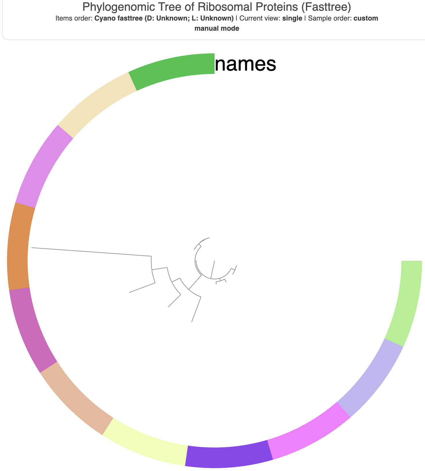
The tree visualization before any adjustments.
Those colors aren’t very helpful labels for the tips of the tree, and since we have only a few genomes, we can turn this circular visualization into a more conventional flat one. To make these changes in the interface Settings panel, you can do the following (remember to click ‘Draw’ afterwards to see the effect):
- under the ‘Items’ section, change ‘Drawing Type’ from ‘Circle Phylogram’ to ‘Phylogram’
- also change the ‘names’ display type from ‘Color’ to ‘Text’
- to remove the gray background from behind the names, adjust the leftmost color box for ‘names’ to be white (hex code
#ffffff) - while you are changing the settings, note the Scale Bar, which provides the scale for the branch length distance in the tree
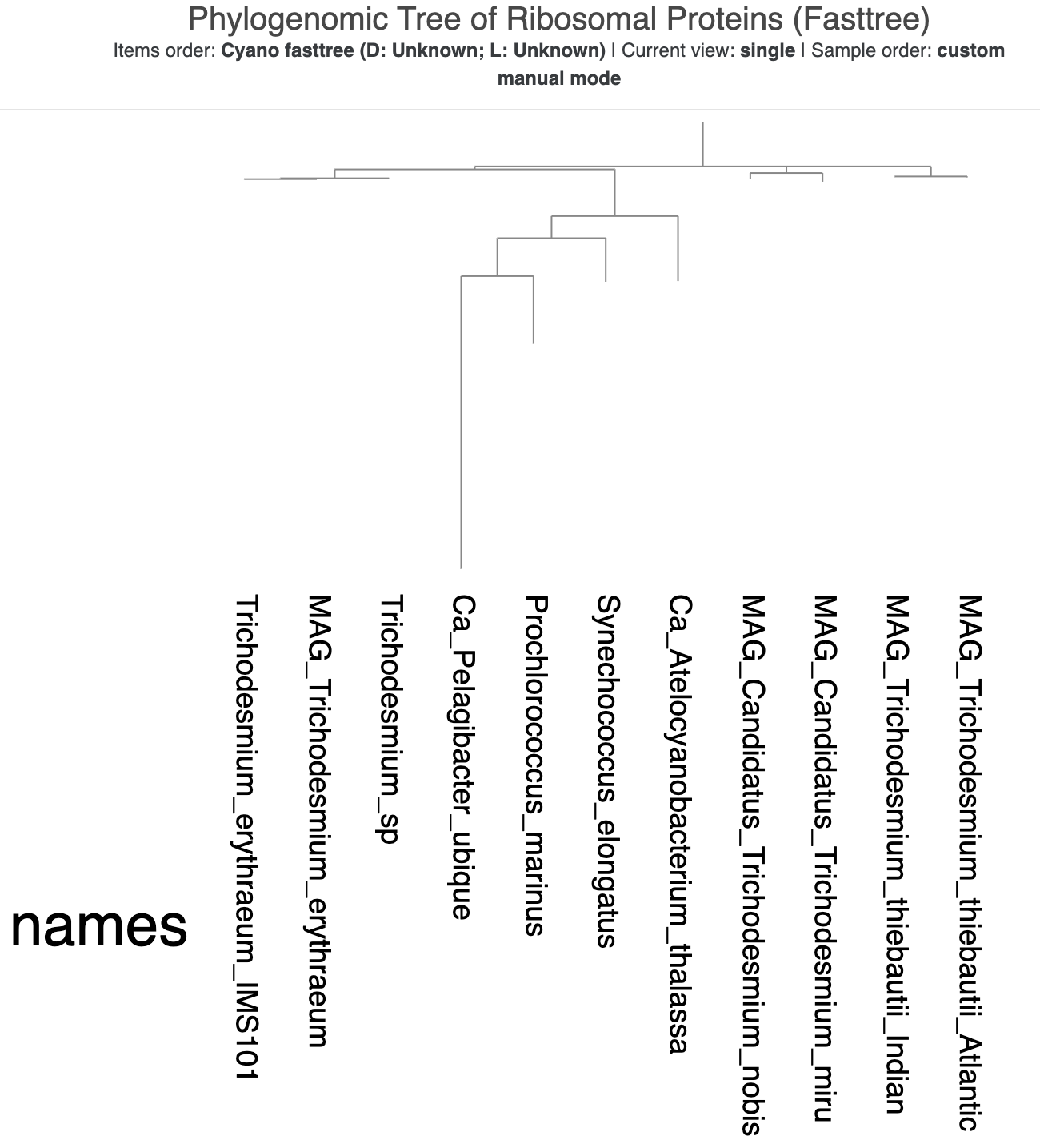
A slightly more readable phylogenomic tree.
That looks much cleaner already. But the tree might look a bit weird to you – what is with that long branch in the middle of it?
That’s our outgroup! We can root the tree on that longest branch to make it the outermost branch of the tree and bring all the cyanobacteria together. Right-click on the Ca. Pelagibacter ubique (SAR11) branch and select “Reroot”. The tree should now look like this:
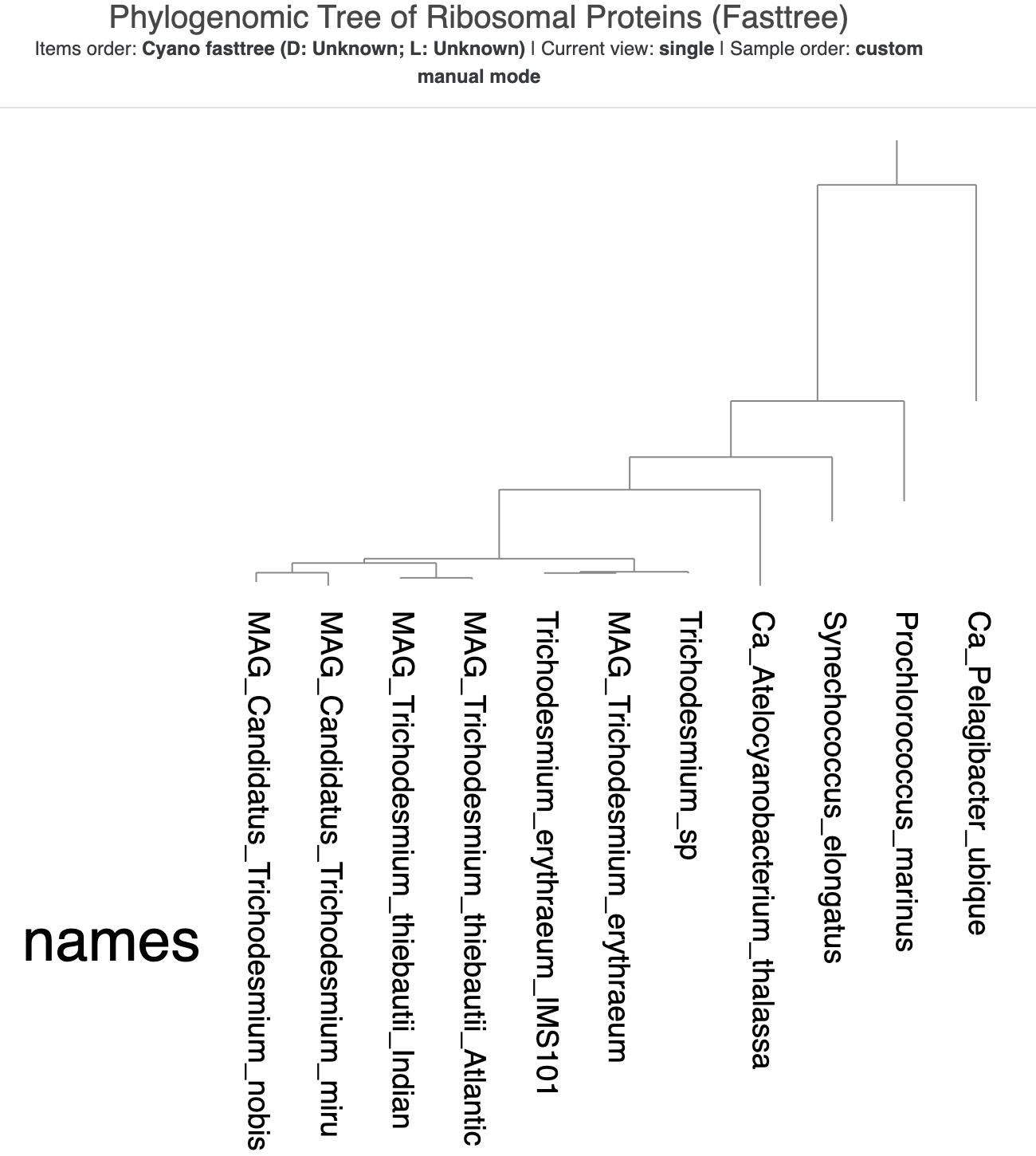
The rooted version of the tree.
Now we can actually make some conclusions about the evolutionary relationships between the cyanobacteria. First, our favorite candidate species T. nobis and T. miru are more closely related to each other than to the other Trichodesmium species. This matches their arrangement in the pangenomic dendrogram in the previous chapter. Second, the Trichodesmium sp. MAG that we added to Tom Delmont’s original set of genomes is placed with the other T. erythraeum genomes, which matches our earlier taxonomic prediction for this MAG. It is really nice when all the evidence points to the same result.
As for how Trichodesmium relates to the other cyanobacterial celebrities that we have in this tree, the tree tells us that Ca. Atelocyanobacterium thalassa is the most closely-related to Trichodesmium of the three, followed by Synechococcus elongatus and then Prochlorococcus marinus. That largely makes sense given our current taxonomic knowledge about cyanos, especially considering that the phylogenomic tree of the Cyanobacteriales order in Tom’s paper (Supplementary Figure 1) includes UCYN-A1, a sublineage of Ca. Atelocyanobacterium thalassa. Check out that figure below for comparison:
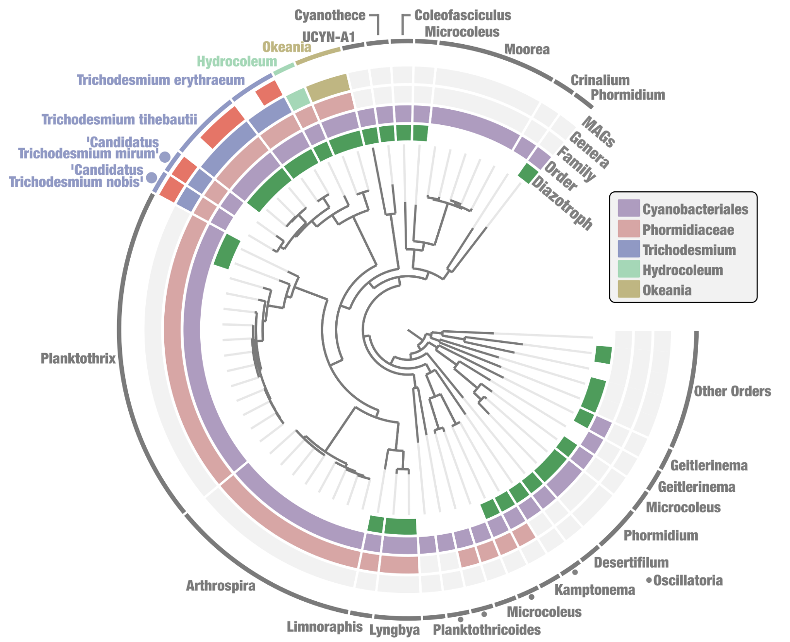
Supplementary Figure 1 of Delmont 2021 – A phylogenomic tree of Cyanobacteriales genomes.
If you focus in on the Trichodesmium genomes in that figure, you will see that it shows the same arrangement as the basic little tree that we just made. :)
Tom’s tree contains much more information though, as it includes additional layers describing whether each genome is a MAG (red) or not, the higher-level taxonomic groups that some of the genomes belong to, and whether the genome has nitrogen-fixing capacity (the green ‘diazotroph’ layer) or not. We can make our tree include additional information like that, too. But before we do that, let’s go through one additional method for inferring a phylogenomic tree.
Before you quit the interactive interface in the terminal by hitting CTRL-C, don’t forget to save your visualization settings in a ‘state’ by clicking the ‘Save’ button on the bottom left of the screen, since we’ll re-use them for the next tree. The settings will be stored in the profile database. If you name the state ‘default’, then the saved visualization settings will automatically be loaded the next time we open the interface using the same profile database. And if you also want to save the changes you made to the tree itself (the re-rooting), you should use the ‘Save’ button in the main Settings panel to do so.
Making another tree with IQ-Tree
Another popular software for inferring phylogenomic trees is IQ-Tree, and one thing that it does differently from FastTree is that it does ‘bootstraps’ – it repeats the tree inference multiple times so that it can build a consensus tree combining the most commonly-observed features across all of the bootstrap trees. This also allows it to estimate how accurate each inferred branch is based on the proportion of times that arrangement was observed in the bootstraps; we call these accuracy estimates ‘branch support values’.
Another perk of IQ-Tree is that it allows you to specify the outgroup, meaning that we won’t have to fuss with re-rooting the tree ourselves later.
To demonstrate these advantages, we’ll use IQ-Tree to make another phylogenomic tree using the same concatenated sequence alignment of our ribosomal proteins as before. This time, we’ll use a different model for amino acid evolution, the WAG model.
One additional step that many people often take before inferring phylogenomic trees is to remove positions with too many gaps from the concatenated alignment. When a majority of genomes have a gap character at the same exact position in the alignment, it can indicate poor alignment or spurious sequences that introduce noise into the evolutionary signal. We aren’t removing these gap-heavy positions in this tutorial because there aren’t enough of them to make a difference in the final tree inference. But just for an example, one software you can use for this is Trimal, and an example command to remove positions with over 50% gaps in our dataset would be: trimal -in 02_PHYLOGENOMICS/RP_sequences.fa -out RP_sequences_GAPS_REMOVED.fa -gt 0.50.
# takes ~15 seconds to run
iqtree -s 02_PHYLOGENOMICS/RP_sequences.fa \
       -T 4 \
       -m WAG \
       -B 1000 \
       -o Ca_Pelagibacter_ubique \
       --prefix 02_PHYLOGENOMICS/cyano_iqtree
In the IQ-Tree command above, -T is the number of threads, -m indicates the evolutionary model to use, -B is the number of bootstrap replicates to run, -o specifies our outgroup genome, and --prefix is the prefix of all output files that will be generated by the software.
IQ-Tree will work quite quickly and produce a lot of output on your terminal, but at the bottom you should see a nice summary of the outputs. In particular, you will notice that the ‘consensus tree’ was written to a file called 02_PHYLOGENOMICS/cyano_iqtree.contree. Let’s use the anvi’o interactive interface to visualize this new tree, using the same profile database as before:
anvi-interactive --tree 02_PHYLOGENOMICS/cyano_iqtree.contree \
                 -p 02_PHYLOGENOMICS/phylo-profile.db \
                 --title "Phylogenomic Tree of Ribosomal Proteins (IQ-Tree)" \
                 --manual
This time, because we saved the state from our previous tree, you should immediately see the ‘cleaner’ version of the visualization, with text labels instead of colors and the rectangular format. But something is up with the tree root! It looks like the root is made up of two genomes – both Ca. Pelagibacter ubique and Prochlorococcus marinus – instead of just SAR11.
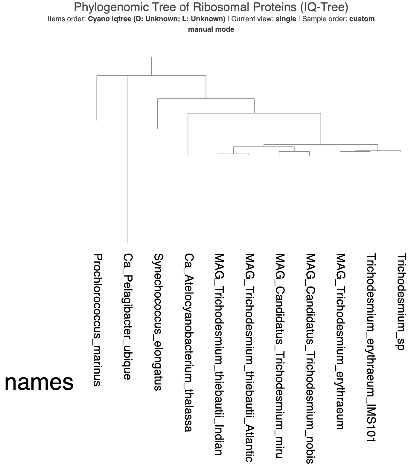
The new tree made with IQ-Tree, visualized using the same state as the previous tree.
To investigate what happened here, scroll back up in your terminal to the IQ-Tree output and take a look through the entire thing. You should eventually find a hint of what happened in this section:
                                       Gap/Ambiguity  Composition  p-value
Analyzing sequences: done in 2.98023e-05 secs using 295.3% CPU
   1  Trichodesmium_sp                        10.94%    passed     99.76%
   2  Synechococcus_elongatus                 13.84%    failed      0.00%
   3  MAG_Candidatus_Trichodesmium_nobis      12.83%    passed     99.44%
   4  MAG_Trichodesmium_thiebautii_Atlantic   17.42%    passed     78.26%
   5  Ca_Pelagibacter_ubique                   9.88%    failed      0.00%
   6  Trichodesmium_erythraeum_IMS101         11.14%    passed     99.64%
   7  MAG_Trichodesmium_thiebautii_Indian     12.73%    passed     94.38%
   8  MAG_Candidatus_Trichodesmium_miru       10.28%    passed     99.77%
   9  Ca_Atelocyanobacterium_thalassa         13.37%    passed     90.19%
  10  Prochlorococcus_marinus                 11.56%    failed      0.00%
  11  MAG_Trichodesmium_erythraeum            10.90%    passed     99.66%
****  TOTAL                                   12.26%  3 sequences failed composition chi2 test (p-value<5%; df=19)
The IQ-Tree FAQ explains what this ‘Composition Test’ means:
At the beginning of each run, IQ-TREE performs a composition chi-square test for every sequence in the alignment. The purpose is to test for homogeneity of character composition (e.g., nucleotide for DNA, amino-acid for protein sequences). A sequence is denoted failed if its character composition significantly deviates from the average composition of the alignment.
Our three non-Cyanobacteriales genomes failed the composition test, meaning that their ribosomal protein sequences were significantly different from those of the Cyanobacteriales. That makes biological sense, and also helps explain why the root now contains two genomes. Based on our earlier tree from FastTree, we know that P. marinus was the most closely-related to our SAR11 genome. Their RPs must have been so similar, and so different from the Cyanobacteriales genomes, that IQ-Tree put them together in the root.
That’s all fine, but because the multi-genome root looks a bit weird (and because we know that SAR11 is in a completely different taxonomic class and phylum from the rest of the microbes), we are going to force the SAR11 genome to the outside by re-rooting at the Ca. Pelagibacter ubique branch like we did before. When you right-click, be sure to choose the option ‘Reroot (preserve support values)’ to make sure any support values are moved along with their branches.
Afterwards, the tree should look like this instead:
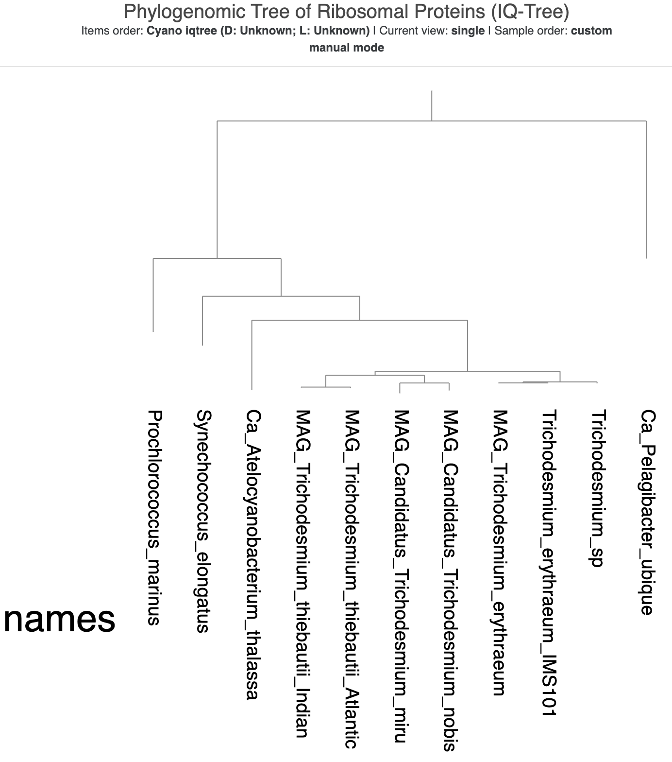
The re-rooted phylogenomic tree from IQ-Tree.
That very long distance between SAR11 and P. marinus is now a bit awkward. Luckily, we can do horizontal rotations of branches in the tree because these don’t affect the inferred evolutionary relationships in the tree. Right-click on the branch leading to the division between P. marinus and the rest of the genomes (besides SAR11), and select the option ‘Rotate the tree/dendrogram here’. That should flip the rest of the branches so that the tree now looks like a staircase, with the Trichodesmium genomes all the way on the left:
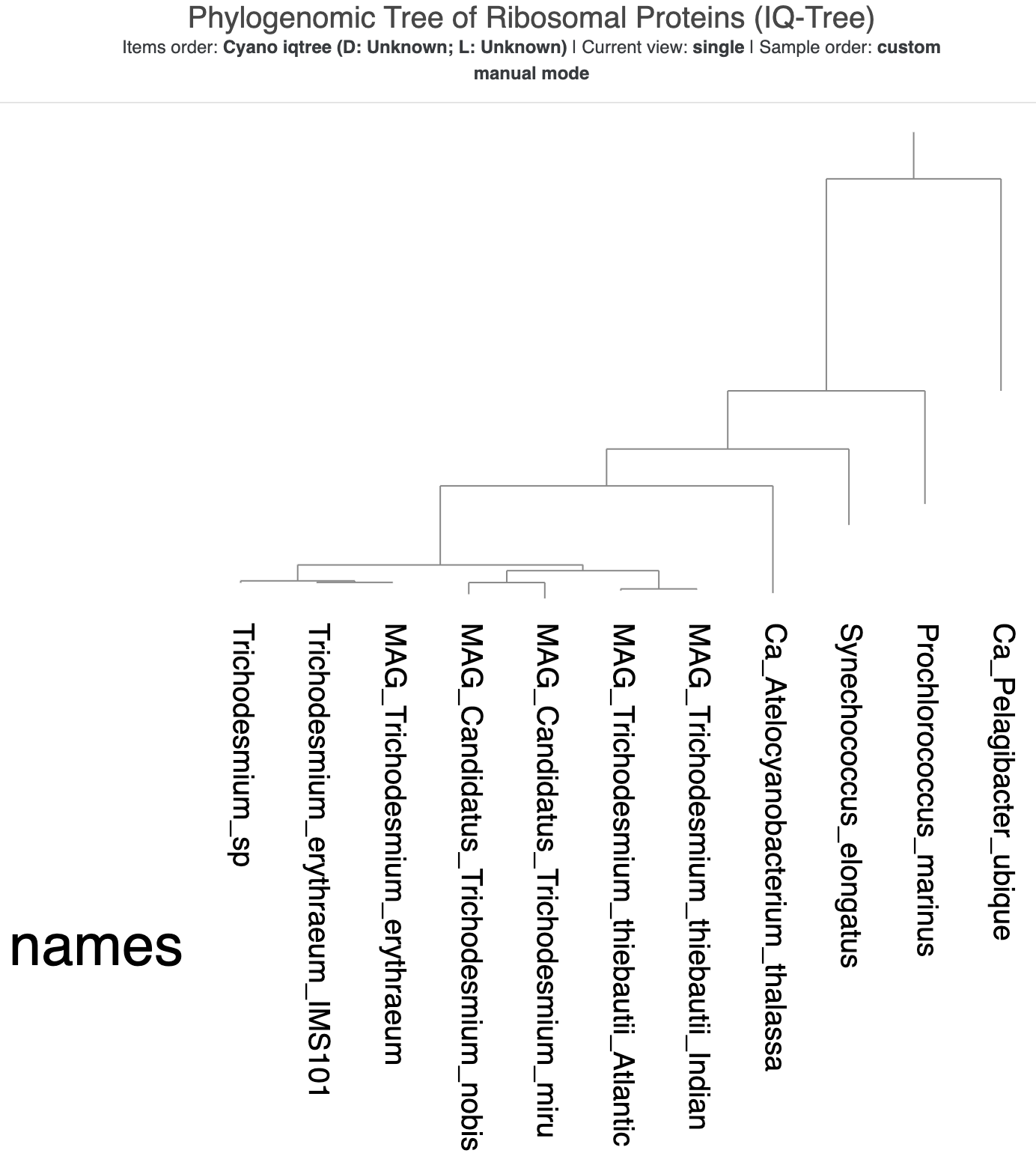
The re-rooted and rotated phylogenomic tree from IQ-Tree.
If you compare it to the FastTree version from before, you will see that it has the exact same topology/arrangement of branches (ignoring any horizontal re-arrangements). However, the branch lengths are slightly different - you cannot really tell from the visualization itself, but if you look in the Settings panel on the left, you will see that the scale bar value is different from before.
Now let’s add the branch support values. In the Settings panel on the left, click on the ‘Options’ tab and find the ‘Branch Support’ section. There, check the box next to ‘Display’, and also check the box for either ‘Symbols’ or ‘Text’ to choose the format of the branch support visualization. If you use the ‘Symbols’ option, you can change the ‘Symbol Size Range’ to make the symbols larger (I set the upper value to 20). If you use the ‘Text’ option, it may be a good idea to increase the font size value and set the ‘Text Rotation’ value to 270 so that the values are written horizontally rather than sideways.
When you click the ‘Draw’ button again, you should now see that the branch points are annotated with either circles of various sizes (the bigger, the better) or text indicating the proportion of bootstrap trees with the same arrangement:
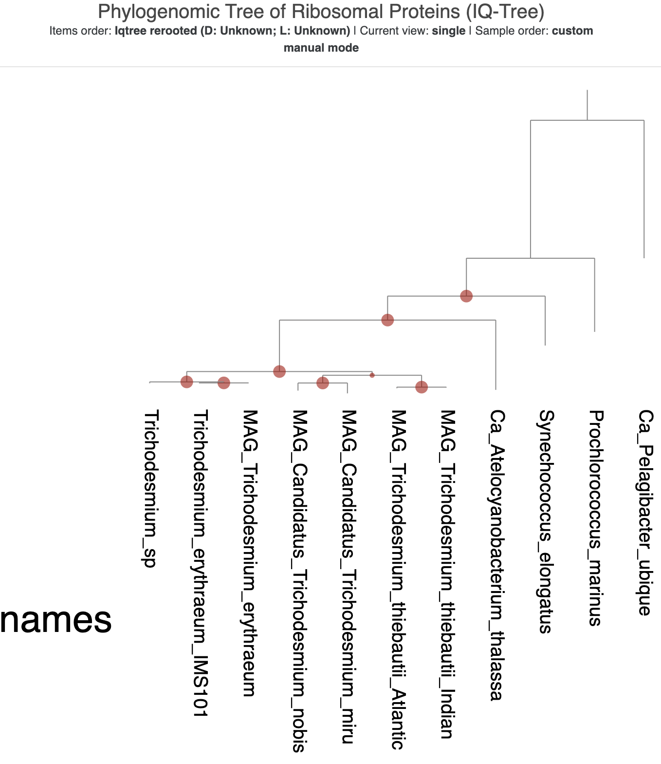
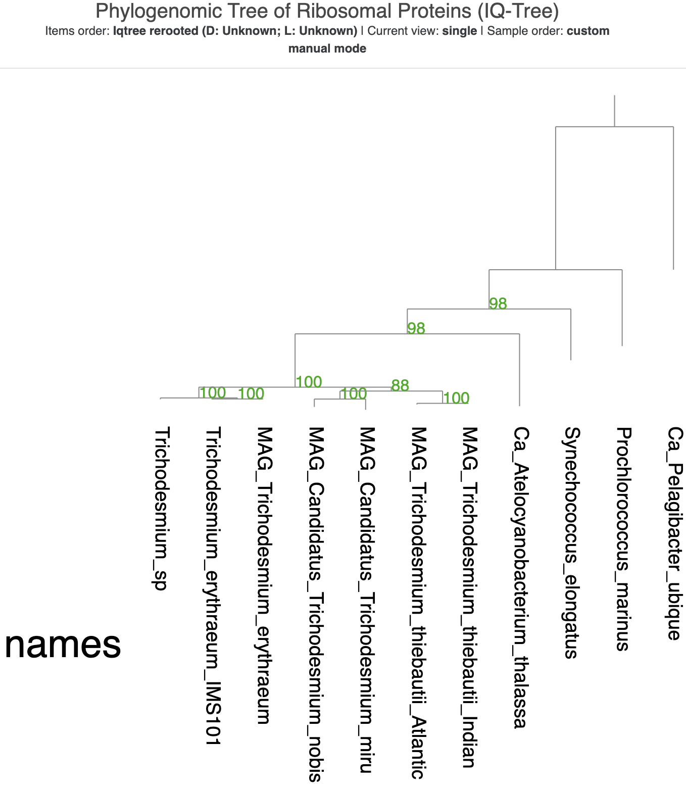
You can see that most of the branches have good support values. The outermost two branches are the only ones without support values. A root of a phylogenomic tree typically gets a null support value, and since IQ-Tree placed both SAR11 and P. marinus at the root, both of their branches lack any support value (even after we explictly made SAR11 the root).
Adding misc data to the tree
Our next task is to enhance the visualization with some additional data about each genome in the tree. Before you quit the interactive interface, don’t forget to save your state and the changes to the phylogenomic tree.
We’re going to add some taxonomic information to the tree so that we can make layers showing the Order and Class of each microbe. We’re also going to highlight the diazotrophs with nitrogen-fixing capacity (as indicated by the presence of nifHDK genes).
To get the GTDB-based taxonomy estimates, we’ll run anvi-run-scg-taxonomy on our external-genomes file like we did in Chapter 1:
anvi-estimate-scg-taxonomy -e 02_PHYLOGENOMICS/external-genomes-phylogenomics.txt -o 02_PHYLOGENOMICS/taxonomy_phylogenomics.txt
If you look at the output file, you may notice that the first column, name, has the same ID for each genome as the labels on the phylogenomic tree. That will be important for the interface to assign the additional data to the correct branch later.
name |
total_scgs |
supporting_scgs |
t_domain |
t_phylum |
t_class |
t_order |
t_family |
t_genus |
t_species |
|---|---|---|---|---|---|---|---|---|---|
| MAG_Candidatus_Trichodesmium_miru | 22 | 15 | Bacteria | Cyanobacteriota | Cyanobacteriia | Cyanobacteriales | Microcoleaceae | Trichodesmium | Trichodesmium sp023356515 |
| MAG_Candidatus_Trichodesmium_nobis | 20 | 13 | Bacteria | Cyanobacteriota | Cyanobacteriia | Cyanobacteriales | Microcoleaceae | Trichodesmium | Trichodesmium sp023356535 |
| MAG_Trichodesmium_erythraeum | 22 | 21 | Bacteria | Cyanobacteriota | Cyanobacteriia | Cyanobacteriales | Microcoleaceae | Trichodesmium | Trichodesmium erythraeum |
| MAG_Trichodesmium_thiebautii_Atlantic | 21 | 21 | Bacteria | Cyanobacteriota | Cyanobacteriia | Cyanobacteriales | Microcoleaceae | Trichodesmium | Trichodesmium sp023356605 |
We probably won’t want to display all of these columns of data in the interface, but it doesn’t hurt to keep them in the file.
To identify which of our genomes have the classic marker gene for nitrogen fixation, nifH, we can use anvi-search-functions on the same external-genomes file. If you followed earlier chapters of this tutorial, you might recall that we only trust KOfam annotations for this gene because some NCBI COG annotations for the nifH gene were incorrect; therefore, we only allow matches from the KOfam annotation source:
anvi-search-functions -e 02_PHYLOGENOMICS/external-genomes-phylogenomics.txt \
    --search-terms NifH \
    --annotation-source KOfam \
    -o 02_PHYLOGENOMICS/NifH_matches.txt
The output looks like this:
item |
genome |
NifH_hits |
|---|---|---|
| GCF_000025125_000000000001_split_00035 | Ca_Atelocyanobacterium_thalassa | NifH |
| TARA_PON_SSUU_QQSS_MMQQ_GGZZ_GGMM_000000996978_split_00001 | MAG_Trichodesmium_erythraeum | NifH |
| TARA_AON_SSUU_QQSS_MMQQ_GGZZ_GGMM_000005288253_split_00001 | MAG_Trichodesmium_thiebautii_Atlantic | NifH |
| TARA_IOS_SSUU_QQSS_QQRR_MMQQ_GGQQ_GGMM_000002452605_split_00001 | MAG_Trichodesmium_thiebautii_Indian | NifH |
The first column is the split name on which at least one gene with a matching annotation was found. The split names aren’t useful for our purposes right now, but would be useful if you wanted to import items additional data into a contigs database visualization (in which the items are splits). What we care about at the moment is the genome column, because that column will match the item names in our phylogenomic tree. The last column(s) in the file will contain each search term we used, and will be non-empty only if that search term was found on a given split – although in our case, because we used only a single search term, all of the rows have NifH in the final column.
What we want to do is add the search result column to our earlier taxonomy table. We’ll go through the genome names in that table one by one and look for them in our search results, creating a new column of True/False values indicating whether each genome had a nifH match or not.
In addition, we want to keep the branch tip labels in the visualization, but these unfortunately go away when visualizing additional data in the interface. To keep them around, we’ll also add a column of the branch labels to our additional data file, so that it effectively becomes an additional data layer itself. Then we’ll put those two new columns together with the taxonomy table to make a misc-data-items-txt file:
echo -e "NifH\tname" > 02_PHYLOGENOMICS/nif_matches.txt
while read genome other_fields
do
  if grep -q $genome 02_PHYLOGENOMICS/NifH_matches.txt
  then
    echo -e "True\t$genome" >> 02_PHYLOGENOMICS/nif_matches.txt;
  else
    echo -e "False\t$genome" >> 02_PHYLOGENOMICS/nif_matches.txt;
  fi
done < <(tail -n+2 02_PHYLOGENOMICS/taxonomy_phylogenomics.txt)

# put it all together
paste 02_PHYLOGENOMICS/taxonomy_phylogenomics.txt 02_PHYLOGENOMICS/nif_matches.txt > 02_PHYLOGENOMICS/misc_data_phylogenomics.txt
The resulting file can be added to the phylogenomics visualization using the -d (--view-data) flag, like this:
anvi-interactive --tree 02_PHYLOGENOMICS/cyano_iqtree.contree \
                 -p 02_PHYLOGENOMICS/phylo-profile.db \
                 --title "Phylogenomic Tree of Ribosomal Proteins (IQ-Tree)" \
                 --manual \
                 -d 02_PHYLOGENOMICS/misc_data_phylogenomics.txt
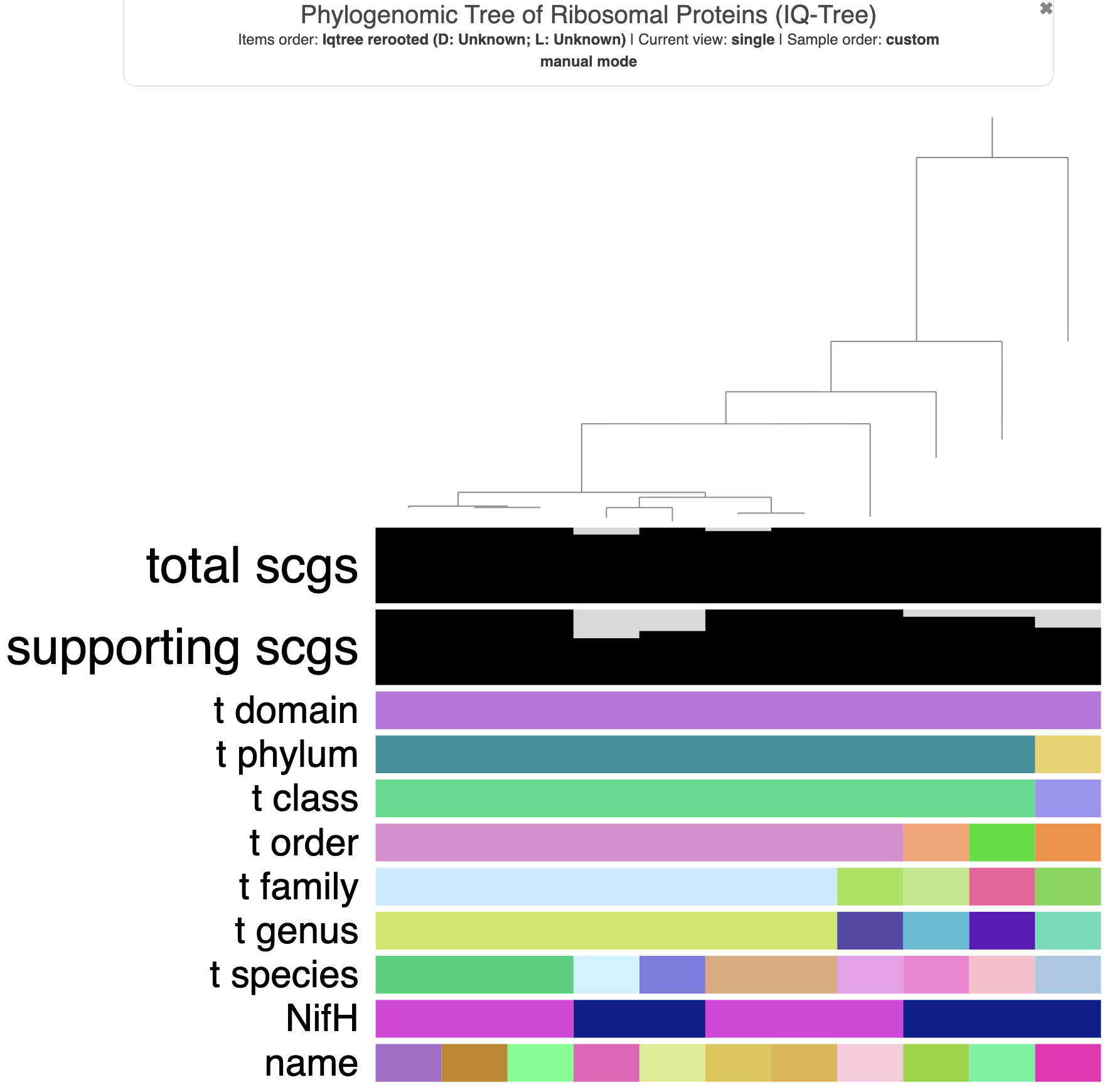
The tree with additional data layers.
If the tree that loads automatically isn’t re-rooted, you likely need to load the rooted version (that you hopefully saved before closing the interface last time). In the Settings panel under the ‘Items’ section, click the dropdown box called ‘Order’ to select your rooted tree, and then re-Draw.
Well. This is a lot of extra layers of data. We don’t want to display all of them, so we’ll remove some. Here are the steps you can take to refine the visualization:
- In the ‘Display’ settings for ‘Items’, set the ‘Height’ attribute to 0 for
total_scgs,supporting_scgs,t_domain,t_phylum, andt_species - Drag the
NifHlayer to the very top so that it is the closest to the tree tips. - Increase the ‘Margin’ attribute for
t_classand forNifHto 50 and 100, respectively. This will add some extra white space in between the tree and theNifHdata, as well as in between theNifHdata and the taxonomy information. - Change the
namelayer from ‘Color’ to ‘Text’ and make the background color of the text white. - Scroll down in the Settings panel to the ‘Legends’ section, and change the colors for the
NifHlayer so that a value of ‘False’ is displayed in white. Feel free to change the color for ‘True’ values as well, if you want. I made them green to mimic Tom’s supplementary figure. - Change the outgroup’s color to white (or off-white) in all the taxonomic layers that we are displaying. The outgroup is only there to root the tree and we don’t want to clutter up the visualization with its obviously different taxonomic information.
- While you are still in the ‘Legends’ section, feel free to change the colors of the other taxonomic groups, if you’d like. I roughly matched the colors in Tom’s supplementary figure when possible.
- Those labels for the layers are huge. You can make them smaller by modifying going to the ‘Options’ tab in the Settings panel, scrolling down to the ‘Layers/Labels’ section, and reducing the ‘Maximum font size’ value. I set it to 50.
- With T. nobis and T. miru in the middle of the other Trichodesmium genomes, there is a gap in the
NifHlayer that looks a bit strange. You could rotate those branches in the tree to put T. nobis and T. miru on the outside, if you’d like. - Don’t forget to save your state (and your tree, if you rotated any branches).
Here is what the tree looked like when I was done with it:
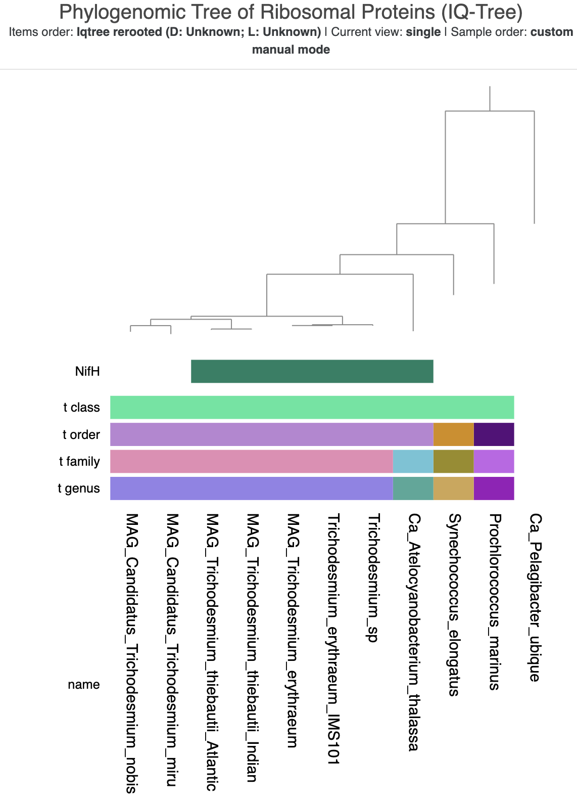
The refined tree visualization with taxonomy and NifH data.
It needs a bit more polishing in an SVG editor like Inkscape to be as pretty as Tom’s figure, but is good enough for our purposes today.
The next chapter
If you want to immediately move on to the next chapter of this tutorial, here is the link:
If you want to go back to the main page of the tutorial instead, click here.
If you have any questions about this exercise, or have ideas to make it better, please feel free to get in touch with the anvi’o community through our Discord server: