An anvi'o tutorial with Trichodesmium genomes (Chapter 5)


Table of Contents
- Quick Navigation
- Read Recruitment
- Getting started
- Mapping one metagenome to a single genome
- Mapping many metagenomes to a single genome
- Visualizing read recruitment data
- Non-competitive read recruitment (mapping many metagenomes to many genomes in individual FASTA files)
- Competitive read recruitment (mapping many metagenomes to many genomes in ONE combined FASTA file)
- What we’ve learned
- Congrats!
About this page This webpage is one chapter of a much larger effort to cover multiple aspects of anvi’o in the same tutorial. If you need more context, please visit the main page of the tutorial, where you will find information about the dataset we are working with and the commands to download the tutorial datapack.
Quick Navigation
- Tutorial introduction (main page)
- Chapter 1: Genomics
- Chapter 2: Pangenomics
- Chapter 3: Phylogenomics
- Chapter 4: Metabolism
- Chapter 5: Read Recruitment ← you are here
Read Recruitment
Show/Hide Starting the tutorial at this section? Click here for data preparation steps.
If you haven’t run previous sections of this tutorial, then you should follow these steps to setup the files that we will use going forward.
cp 00_DATA/contigs/*-contigs.db .
anvi-script-gen-genomes-file --input-dir . -o external-genomes.txt
Read recruitment, or read mapping, is a critical step in most metagenomics projects. It allows us to compute coverage and detection statistics, enabling us to (1) estimate an organism’s relative abundance and presence-absence in samples, (2) analyze biogeography, and (3) more accurately bin contigs into metagenome-assembled genomes (MAGs). It also allows us to identify sequence variants and insertions/deletions, enabling us to do population genetics.
This chapter of the tutorial covers read recruitment for the case when you have genome(s) to map reads to (that is, the genomes will be your reference sequences). We’ll use the results to (roughly) analyze the biogeography of our four Trichodesmium species. That said, the commands for mapping are similar if you use different types of reference sequences such as a metagenomic assembly (for instance, if you want to get differential coverage for binning) or individual genes (for instance, if you want to analyze the distribution of functions across samples).
There are many bioinformatic tools for recruiting reads, like Bowtie 2, BWA, Strobealign, and Minimap2. Anvi’o is not one of them, but it does include several programs to process the output of read recruitment – specifically, BAM files. And mapping reads is such a common task that the anvi’o metagenomics workflow includes all the steps for read recruitment. Therefore, several 3rd-party software options for read recruitment are typically installed within your anvi’o conda environment, so you should have access to them.
In this chapter, we will learn how to do the following tasks that don’t involve anvi’o programs:
- mapping metagenomic reads to a reference using Bowtie 2
- processing the mapping output files using SAMtools
- setting up competitive or non-competitive read recruitment
In addition, we will learn how to process the read recruitment results within anvi’o:
- computing coverage, detection, and single-nucleotide variants (SNVs)
- visualizing read recruitment data in the interactive interface
Getting started
In your terminal, you should be located within the trichodesmium_tutorial folder. From there, you can check the contents of the 00_DATA/mapping folder:
$ ls 00_DATA/mapping/
ATLANTIC_R1.fastq.gz  BACKUP_PROFILES      INDIAN_OCEAN_R1.fastq.gz  map_competitive.sh     MEDITERRANEAN_R1.fastq.gz  PACIFIC_R1.fastq.gz  RED_SEA_R1.fastq.gz  samples_info.txt  tricho_sp_state.json
ATLANTIC_R2.fastq.gz  combined_state.json  INDIAN_OCEAN_R2.fastq.gz  map_noncompetitive.sh  MEDITERRANEAN_R2.fastq.gz  PACIFIC_R2.fastq.gz  RED_SEA_R2.fastq.gz  samples.txt
You should see 5 metagenome samples named according to where they were sampled. Note that these were derived from publicly-available metagenomes sampled during the Tara Oceans cruise (Sunagawa et al 2015). The original samples were subsetted to make them small enough to work with on a typical laptop. If you want to know the BioSample accessions of the original samples, you can check the samples_info.txt file in the same folder.
To keep things organized as we start generating read recuitment data, we will make ourselves a sub-directory to work in:
mkdir -p 03_READ_RECRUITMENT && cd 03_READ_RECRUITMENT
And since we’ll be covering two setups for read recruitment – non-competitive and competitive – we will also generate a subfolder for the output of each setup:
mkdir -p NON_COMPETITIVE
mkdir -p COMPETITIVE
We’ll mainly work in the 03_READ_RECRUITMENT directory and direct our output into these last two folders.
Mapping one metagenome to a single genome
We will start with the simplest case: one metagenome sample mapped to one genome. Suppose we want to know whether our Trichodesmium sp. MAG (which was obtained from a Red Sea metagenome) is detectable within the RED_SEA sample in our datapack.
Read recruitment is done from FASTQ files (of reads) to FASTA files (of reference sequences, usually contigs). If you worked through Chapter 1, you already have a FASTA file for this genome that we could use as the reference. However, you might remember that we reformatted the contig names before making our contigs database. It is very important to use a FASTA file in which the contig names match those within the contigs-db, so that anvi’o later knows how to connect the read recruitment results to the right contigs. Therefore, just to be on the safe side, we are actually going to export the contig sequences directly from the contigs database to ensure we are using a FASTA file with the right contig names:
anvi-export-contigs -c ../Trichodesmium_sp-contigs.db -o Trichodesmium_sp.fa
Now that we have a reference FASTA file, our first step is to index it. Indexing makes the mapping step faster.
bowtie2-build Trichodesmium_sp.fa Trichodesmium_sp
Notice what files were created in your working directory.
We can now use the index files to map reads from our metagenome sample of interest. This particular sample comes from the Red Sea – it is not the same sample from which our downloaded MAG was reconstructed, but if it contains a similar-enough population then our MAG’s contigs will be able to recruit reads from that ‘local analogue’ of Trichodesmium sp.
Mapping to a single genome is considered ‘non-competitive’ read recruitment because the sequencing reads only have one biological entity to map to – if there were other genomes in the reference FASTA file, then the genomes would be competing with each other to recruit reads and sequences of highly similar or shared genomic regions would be drawn to the genome they are most similar to. But there is only one genome in our current index, so we’ll direct the mapping output to the NON_COMPETITIVE folder. Here is the mapping command:
bowtie2 -x Trichodesmium_sp \
        -1 ../00_DATA/mapping/RED_SEA_R1.fastq.gz \
        -2 ../00_DATA/mapping/RED_SEA_R2.fastq.gz \
        -S NON_COMPETITIVE/RED_SEA-Trichodesmium_sp.sam
We’ve named the output file with the metagenome’s BioSample accession combined with the genome name because later, we’ll be mapping the same sample to different references.
In the terminal output from Bowtie, you should see some information about how many reads were able to map to the genome. It is not 100% because the metagenome includes DNA from organisms that are not similar enough to the reference to be able to map. Another way to interpret the line 45.58% overall alignment rate is “your reference for mapping includes ~45% of the community captured in the metagenome”.
If you’ve never seen a SAM file before, it’s worth it to take a look at NON_COMPETITIVE/RED_SEA-Trichodesmium_sp.sam using less to understand what sort of information it includes. Here’s a link to the SAM file Wikipedia page, which has a nice explanation of the format.
SAM files take up a lot of space, so we want to convert them to smaller binary files (BAM). To further save on space, we can exclude unmapped reads from the BAM file (this is what the -F 4 option does below). Then, to make the BAM file faster to process, we (1) sort and (2) index it. All of this is done with SAMtools using these commands:
samtools view -F 4 \
              -bS NON_COMPETITIVE/RED_SEA-Trichodesmium_sp.sam \
              -o NON_COMPETITIVE/RED_SEA-Trichodesmium_sp-RAW.bam

samtools sort NON_COMPETITIVE/RED_SEA-Trichodesmium_sp-RAW.bam -o NON_COMPETITIVE/RED_SEA-Trichodesmium_sp.bam
samtools index NON_COMPETITIVE/RED_SEA-Trichodesmium_sp.bam
If all of that was successful, you should see the sorted BAM file RED_SEA-Trichodesmium_sp.bam and its corresponding index (.bai) file in the output directory. Then you are free to remove the original SAM file and the unsorted BAM:
rm NON_COMPETITIVE/RED_SEA-Trichodesmium_sp.sam NON_COMPETITIVE/RED_SEA-Trichodesmium_sp-RAW.bam
The anvi’o program anvi-init-bam can take an unsorted BAM file and run the samtools sort and samtools index steps on it. It’s a little shortcut in case you want to type less (but as it is simply a driver for these SAMtools programs, we thought it would be better to show those steps explicitly here).
Now what? Knowing which reads map where is one thing, but what we are really after are read recruitment statistics like coverage and detection. In anvi’o, we call the calculation of these metrics ‘profiling’, and there are a couple of programs to do it. anvi-profile-blitz gives you really basic read recruitment statistics in a tab-delimited text file. It’s very fast and a good option if you are working with a very large number of samples. Meanwhile, anvi-profile not only computes coverage and detection, but also identifies single-nucleotide variants, and stores this information in a profile database that can later be used for visualization in the anvi’o interactive interface. As it is not so interesting to visualize read recruitment data from a single metagenome, we’ll start with the former option:
anvi-profile-blitz -c ../Trichodesmium_sp-contigs.db \
                   -o NON_COMPETITIVE/Tricho_sp_contig_stats.txt \
                   NON_COMPETITIVE/RED_SEA-Trichodesmium_sp.bam
If you look at the output, you will see that the read recruitment metrics have been computed on a per-contig basis.
contig |
sample |
length |
gc_content |
num_mapped_reads |
detection |
mean_cov |
q2q3_cov |
median_cov |
min_cov |
max_cov |
std_cov |
num_windows |
prop_windows_covered |
prop_cov_within_foldrange |
dis_cov |
|---|---|---|---|---|---|---|---|---|---|---|---|---|---|---|---|
| Trichodesmium_sp_MAG_R01_000000000001 | RED_SEA-Trichodesmium_sp | 40296 | 0.349 | 66 | 0.1026 | 0.1647 | 0.0 | 0.0 | 0 | 6 | 0.5971 | 101 | 0.297 | 0.8624 | 0.5797 |
| Trichodesmium_sp_MAG_R01_000000000002 | RED_SEA-Trichodesmium_sp | 7609 | 0.306 | 2 | 0.02418 | 0.02418 | 0.0 | 0.0 | 0 | 1 | 0.1536 | 26 | 0.07692 | 1.0 | 0.5385 |
| Trichodesmium_sp_MAG_R01_000000000003 | RED_SEA-Trichodesmium_sp | 5360 | 0.343 | 0 | 0.0 | 0.0 | 0.0 | 0.0 | 0 | 0 | 0.0 | 18 | 0.0 | 0.0 | 0.0 |
| Trichodesmium_sp_MAG_R01_000000000004 | RED_SEA-Trichodesmium_sp | 5380 | 0.346 | 14 | 0.07305 | 0.2599 | 0.0 | 0.0 | 0 | 9 | 1.212 | 18 | 0.1667 | 0.6921 | 0.4294 |
This MAG is quite fragmented, with many short contigs. There is quite a lot of variability across the contigs’ read recruitment statistics, but overall it seems like few reads mapped to any single contig, yielding low detection and coverage scores. But we want to know whether the genome as a whole is present in this metagenome – how can we get similar statistics for the entire MAG?
If you look at the program help page, you might notice that you could also elect to compute these metrics on a per-gene level or a per-genome level. Let’s do it again to get genome-level stats. We will need to make a collection-txt file to tell anvi’o that all contigs in the contigs database belong to our Trichodesmium sp. genome:
# extract the contig names from the FASTA file (removing the initial '>' character)
grep '>' Trichodesmium_sp.fa | sed 's/>//g' > contigs
# extract the genome name from each contig name (i.e., 'Trichodesmium_sp_MAG_R01_000000000001' becomes 'Trichodesmium_sp_MAG_R01')
cut -d '_' -f 1-4 contigs > genome
# put everything together into a 2-column collection-txt file
paste contigs genome > Trichodesmium_sp_collection.txt
# clean up
rm contigs genome
Then we can generate genome-level stats by adding this collection file to our command:
anvi-profile-blitz -c ../Trichodesmium_sp-contigs.db \
                   -C Trichodesmium_sp_collection.txt \
                   -o NON_COMPETITIVE/Tricho_sp_genome_stats.txt \
                   NON_COMPETITIVE/RED_SEA-Trichodesmium_sp.bam
Now, because we are working with a single genome and a single sample, we get a single line of data in our output file:
bin |
sample |
length |
gc_content |
num_mapped_reads |
detection |
mean_cov |
q2q3_cov |
median_cov |
min_cov |
max_cov |
std_cov |
num_windows |
prop_windows_covered |
prop_cov_within_foldrange |
dis_cov |
|---|---|---|---|---|---|---|---|---|---|---|---|---|---|---|---|
| Trichodesmium_sp_MAG_R01 | RED_SEA-Trichodesmium_sp | 6640707 | 0.34 | 13931 | 0.1063 | 0.2096 | 0.0 | 0.0 | 0 | 53 | 1.01 | 6641 | 0.4575 | 0.8319 | 0.6447 |
Let’s go through the data more systematically this time. A total of ~14,000 reads have mapped to our genome, but only ~21% of the genome is detected in this sample and the overall mean coverage is rather low. In fact, if you look at the coverage values within the interquartile range, they have a mean of 0 (q2q3_cov). This makes sense because less than a quarter of the genome is detected, so of course the middle 50% of per-base coverage values are all zeros. However, that coverage seems to be spread out across about half the genome (prop_windows_covered: ~46% of 1-kb windows have at least some reads mapping to them), and the coverage depth appears roughly stable (prop_cov_within_foldrange: ~83% of the covered bases have a coverage depth within 0.5x to 2x of the median non-zero coverage depth), yielding a distribution of coverage score (discov) of 0.6447. Note that we used default parameters of the distribution of coverage calculation (like the window size and the fold-range of depth) as specified in the anvi-profile-blitz help output.
In anvi’o, the mean of the middle 50% of per-base coverage values is called ‘Q2Q3 coverage’. That is, we throw out the lowest quarter (Q1) and highest quarter (Q4) of per-nucleotide coverages to elimimate any extremely high coverage values, some of which may be due to non-specific read recruitment, and extremely low coverage values, some of which may be due to the absence of individual genes or variable regions in the local population. This leaves only quarter 2 (Q2) and quarter 3 (Q3) of the distribution of all per-nucleotide coverage values, which yield a mean coverage value that can more accurately reflect the population’s true coverage in the sample. Hence, ‘Q2Q3 coverage’. This is a very bad and not statistician-friendly name, we know. Sorry about that.
Taking all that evidence together, it looks like this Red Sea metagenome contains a population that is kind-of similar to the Trichodesmium sp. MAG, but in extremely low abundance. In fact, since our reference contains only a single genome, it is possible that many of these reads originated from different microbial populations (perhaps other Trichodesmium species), but were similar enough to match this genome (i.e., non-specific read recruitment). To find out if this is the case, we’d have to try competitive read recruitment and see if it makes a difference in how many reads map to this MAG (we will do it later).
Why was the read recruitment so limited, given that the MAG originates from the Red Sea? The metagenomes this MAG was generated from and our RED_SEA sample (derived from this metagenome) are very different – the former were sampled in November 2020 from very coastal waters at a depth of 20m in the Gulf of Aqaba (no size fraction information provided), while the latter was sampled in January 2010, much farther south and offshore at a depth of 5m (size fraction 20-180μm). So there are a lot of differences in the sampling and environmental parameters that could contribute to the relative lack of detection of this MAG in our RED_SEA sample. Just because two samples come from the same approximate location does not mean they will contain the same microbes.
Before we move on, let’s use anvi-profile to generate a profile database for this BAM file. We won’t do anything with it right now, but it will come in handy later when we want to visualize this data:
anvi-profile -i NON_COMPETITIVE/RED_SEA-Trichodesmium_sp.bam \
             -c ../Trichodesmium_sp-contigs.db \
             -o NON_COMPETITIVE/RED_SEA-Trichodesmium_sp-PROFILE
If you look in the output directory NON_COMPETITIVE/RED_SEA-Trichodesmium_sp-PROFILE/, you should see a profile database, an auxiliary database, and a log file that recapitulates the terminal output.
Show/Hide What's the difference between a profile database and an auxiliary database?
We are glad you asked. The profile database contains summary statistics like detection, coverage, abundance, etc. for each contig and split as well as the positions and nature of variants like single-nucleotide variants (SNVs), insertions/deletions, single-codon variants (SCVs), and single amino acid variants (SAAVs). Meanwhile, the auxiliary database stores per-nucleotide coverage values – the underlying data that was used to compute the summary statistics.
When you visualize metagenomic data in the interface (we will do this later), the data on the main interface page are the summary statistics taken from the profile database, as discussed in this blog post. But you can also ‘inspect’ individual splits to see the per-nucleotide coverage plots, which are coming from the auxiliary database (with SNV overlays taken from the profile database).
You don’t need the auxiliary database to run anvi-interactive, just the profile database. The auxiliary database will be loaded automatically by anvi’o provided it is located in the same directory as the profile-db. However, if the auxiliary database is not available, you won’t be able to use the ‘inspect’ function in the interface (or run anvi-inspect from the command line).
Mapping many metagenomes to a single genome
We just saw that the Trichodesmium sp. MAG does not have a significant presence in our Red Sea metagenome. So where else could it be? In our datapack, we have one sample from each of several other temperate marine regions, so let’s do a mini-biogeography analysis and see if we can detect this genome in any of the other oceans.
We can repeat the same steps we went through above to map each of our other metagenomes, using the Bowtie 2 index for Trichodesmium sp. that we already created. To make things easy, we’ll use a BASH loop to do this. The datapack contains a samples-txt file containing the relative path to each metagenome – copy this file over, and then loop over each line in the file (skipping the RED_SEA sample we already mapped) to run Bowtie 2, process the output with SAMtools, and anvi-profile:
cp ../00_DATA/mapping/samples.txt .

# this loop should take ~5 minutes to run
while read sample r1 r2
do
  echo "Working on $sample"
  bowtie2 -x Trichodesmium_sp \
        -1 $r1 \
        -2 $r2 \
        -S NON_COMPETITIVE/${sample}-Trichodesmium_sp.sam
  samtools view -F 4 \
        -bS NON_COMPETITIVE/${sample}-Trichodesmium_sp.sam \
        -o NON_COMPETITIVE/${sample}-Trichodesmium_sp-RAW.bam
  samtools sort NON_COMPETITIVE/${sample}-Trichodesmium_sp-RAW.bam -o NON_COMPETITIVE/${sample}-Trichodesmium_sp.bam
  samtools index NON_COMPETITIVE/${sample}-Trichodesmium_sp.bam
  rm NON_COMPETITIVE/${sample}-Trichodesmium_sp.sam NON_COMPETITIVE/${sample}-Trichodesmium_sp-RAW.bam
  anvi-profile -i NON_COMPETITIVE/${sample}-Trichodesmium_sp.bam \
        -c ../Trichodesmium_sp-contigs.db \
        -o NON_COMPETITIVE/${sample}-Trichodesmium_sp-PROFILE
done < <(tail -n+3 samples.txt)
Note that we use tail -n+3 to skip over the header line and the RED_SEA sample (which is the 2nd line) in the samples.txt file. The loop will take several minutes to run, but once it is done, you will have a sorted, indexed BAM file and a single-sample profile database for each sample that was mapped to this genome.
Loops are not the most robust way to scale up this analysis. If one of the commands fails, all the downstream commands for the same sample will fail, too. It would also be a pain to figure out what went wrong without dedicated log files for each step, and you would have to manually re-do the steps that didn’t work. Luckily, there is a much better solution: workflows. More on this later.
Let’s check the MAG’s distribution across all 5 metagenome samples. We can use anvi-profile-blitz on multiple BAM files connected to the same reference. Note that we overwrite the old output file with the help of the --force-overwrite flag:
anvi-profile-blitz -c ../Trichodesmium_sp-contigs.db \
                   -C Trichodesmium_sp_collection.txt \
                   -o NON_COMPETITIVE/Tricho_sp_genome_stats.txt \
                   --force-overwrite \
                   NON_COMPETITIVE/*-Trichodesmium_sp.bam
You should now see 5 lines of data in the output file, one per sample that we mapped to the Trichodesmium sp. genome:
bin |
sample |
length |
gc_content |
num_mapped_reads |
detection |
mean_cov |
q2q3_cov |
median_cov |
min_cov |
max_cov |
std_cov |
num_windows |
prop_windows_covered |
prop_cov_within_foldrange |
dis_cov |
|---|---|---|---|---|---|---|---|---|---|---|---|---|---|---|---|
| Trichodesmium_sp_MAG_R01 | ATLANTIC-Trichodesmium_sp | 6640707 | 0.34 | 63222 | 0.2755 | 0.9557 | 0.05092 | 0.0 | 0 | 137 | 2.422 | 6641 | 0.6698 | 0.606 | 0.6379 |
| Trichodesmium_sp_MAG_R01 | INDIAN_OCEAN-Trichodesmium_sp | 6640707 | 0.34 | 89672 | 0.4043 | 1.358 | 0.3297 | 0.0 | 0 | 330 | 5.24 | 6641 | 0.8765 | 0.8173 | 0.8469 |
| Trichodesmium_sp_MAG_R01 | MEDITERRANEAN-Trichodesmium_sp | 6640707 | 0.34 | 106321 | 0.3289 | 1.591 | 0.1695 | 0.0 | 0 | 723 | 4.992 | 6641 | 0.718 | 0.5518 | 0.6349 |
| Trichodesmium_sp_MAG_R01 | PACIFIC-Trichodesmium_sp | 6640707 | 0.34 | 559968 | 0.9079 | 8.474 | 7.992 | 8.0 | 0 | 404 | 7.665 | 6641 | 0.9858 | 0.7634 | 0.8746 |
| Trichodesmium_sp_MAG_R01 | RED_SEA-Trichodesmium_sp | 6640707 | 0.34 | 13931 | 0.1063 | 0.2096 | 0.0 | 0.0 | 0 | 53 | 1.01 | 6641 | 0.4575 | 0.8319 | 0.6447 |
Funnily enough, our Red Sea-derived Trichodesmium sp. MAG is least detected in our RED_SEA metagenome. It seems to be present in PACIFIC with ~8x coverage, and based on the high distribution of coverage score in INDIAN_OCEAN, it is also confidently present there but in low abundance (~0.3x Q2Q3 coverage). The other samples are on the fence; you could make a case for ‘present but in very low abundance’ or for ‘absent’ depending on how you set thresholds for detection or distribution of coverage.
But it would be much more fun to visualize this data in the interactive interface. We have 5 single-sample profile databases, one for each of the samples we mapped. In order to visualize them in a single display later, we need to merge the data into one profile database using the program anvi-merge:
anvi-merge NON_COMPETITIVE/*-PROFILE/PROFILE.db \
           -c ../Trichodesmium_sp-contigs.db \
           -o NON_COMPETITIVE/TRICHO_SP_MERGED
Now that we have all the data in one file, we no longer need the single-sample profiles, so we can just delete them:
rm -r NON_COMPETITIVE/*-PROFILE/
Visualizing read recruitment data
To view the read recruitment data in the interface, we need the merged profile database and its corresponding contigs-db:
anvi-interactive -c ../Trichodesmium_sp-contigs.db \
            -p NON_COMPETITIVE/TRICHO_SP_MERGED/PROFILE.db \
            --title Trichodesmium_sp
You probably see a display that looks like this:
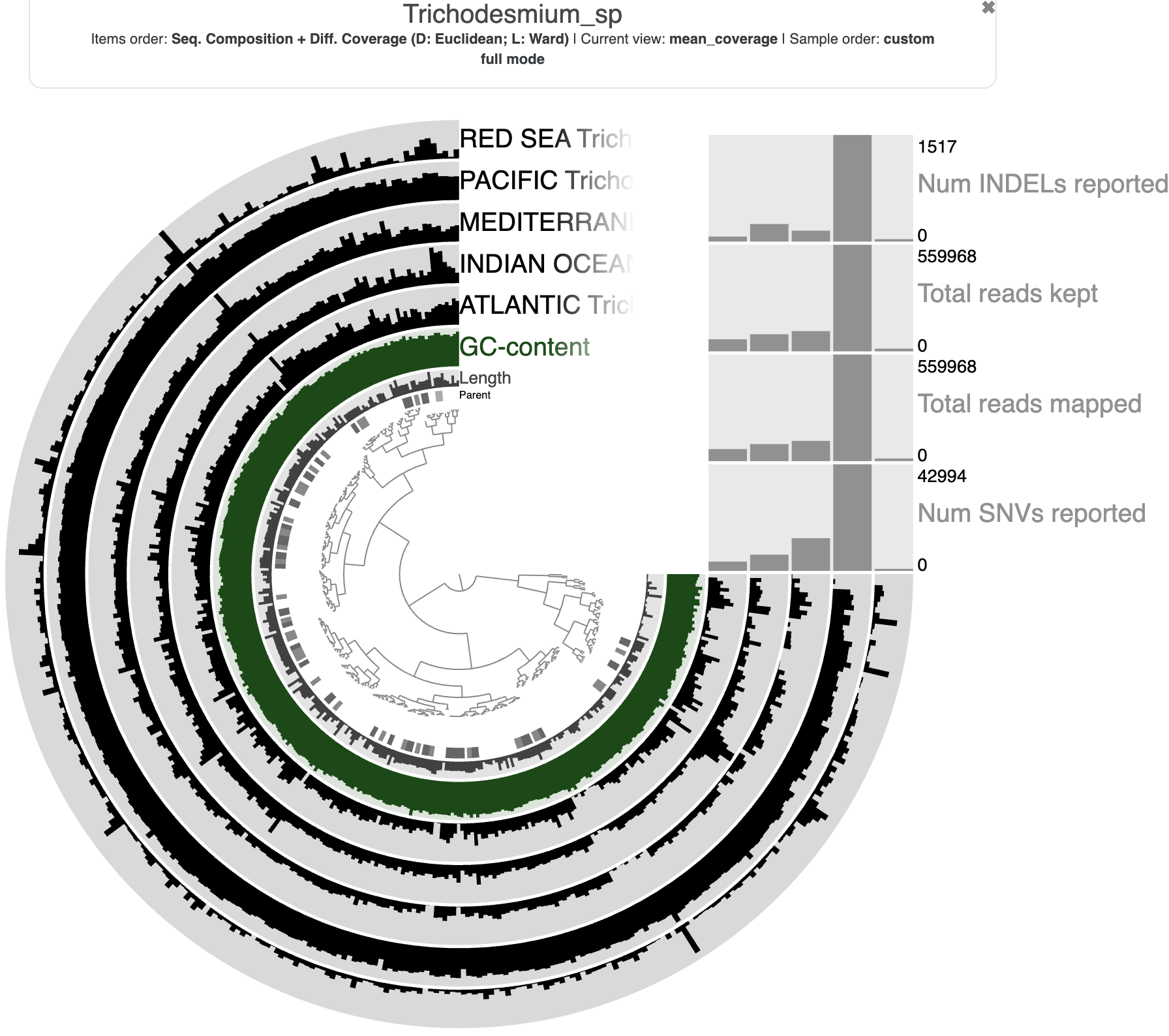
In a metagenomics display, the ‘items’ of the interactive interface are contigs (technically, they are ‘splits’ of contigs so that longer contig sequences take up visual space proportional to their length), and the ‘layers’ are metagenome samples. The first thing to pay attention to is the information at the top of your screen, below the title. It tells you how the genome’s contigs are arranged via the middle dendrogram (here, by their sequence composition and differential coverage across samples), what data we are currently looking at in the layers (at the moment, this is mean coverage), and how the samples are ordered (here, “custom” translates to alphabetical order by sample name).
Another important thing to notice is that the data layers are normalized. In the Settings panel on the left, you should see that the metagenome data layers are log-normalized by default. This normalization is done on a per-sample basis, meaning that each data layer is scaled according to the maximum value within that layer. That is why it appears as though our MAG has plenty of coverage in RED_SEA, even though we know from before that the actual per-contig mean coverage values are very low. You can check the exact coverage values in the ‘Data’ tab by hovering over different layers with your mouse.
Finally, check the additional per-sample (layer) bar plots on the right side. The most reads mapped from the PACIFIC sample and we know that PACIFIC certainly contains a Trichodesmium sp. population, but that doesn’t mean the local population is exactly the same as our MAG – a large number of SNVs and indels were identified from these reads.
Let’s play around with the visualization for a bit. You can change what data is displayed, alter the normalization strategy, change the sample colors, switch the ordering strategy, increase the radius, remove some layers, change the Min/Max of each sample layer, and so on.
Here is what I came up with:
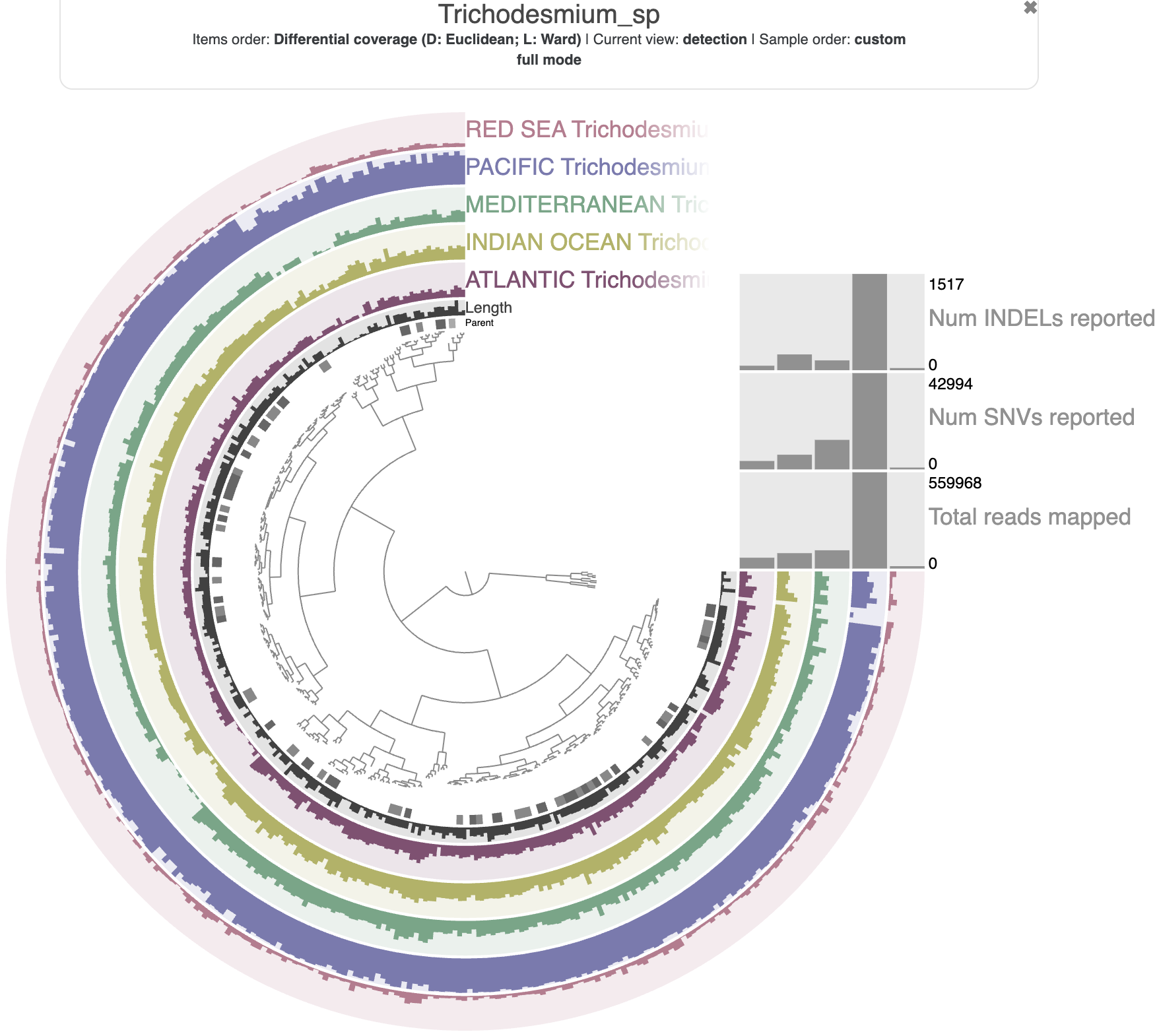
The most important changes I made were:
- switch the data view to ‘Detection’
- enforce all sample layers to have a Min of 0 and a Max of 1 (making the plots comparable across samples)
- order the contigs by ‘Differential coverage’
Along with a few other minor cosmetic things. If you want your display to match mine exactly, you can import the state file provided in the datapack before re-opening the interface and loading the ‘tutorial’ state:
anvi-import-state -p NON_COMPETITIVE/TRICHO_SP_MERGED/PROFILE.db \
            -s ../00_DATA/mapping/tricho_sp_state.json \
            -n tutorial
There are a few things to learn from our display. First, detection is low in most samples (we saw this already in the anvi-profile-blitz output), but now we can see that it is generally consistent within a sample across the entire MAG, meaning that every contig had an approximately similar rate of read recruitment. Second, in the PACIFIC sample there are only a couple of contigs that have 0 detection (on the right), and these are quite short – basically the length of 1-2 genes which must be missing in the local population of this organism.
Let’s inspect one contig to see how the read recruitment patterns look at a finer resolution. We will look at a particularly long contig made up of 8 splits. You can find it by looking for a long gray bar in the ‘Parent’ layer, which indicates all the splits belong to the same contig sequence:
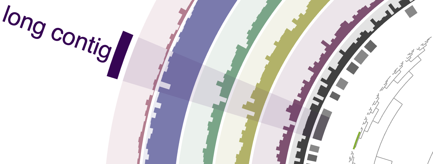
Right-click on any split within that range and hit the ‘Inspect split’ button to open a page like this one:
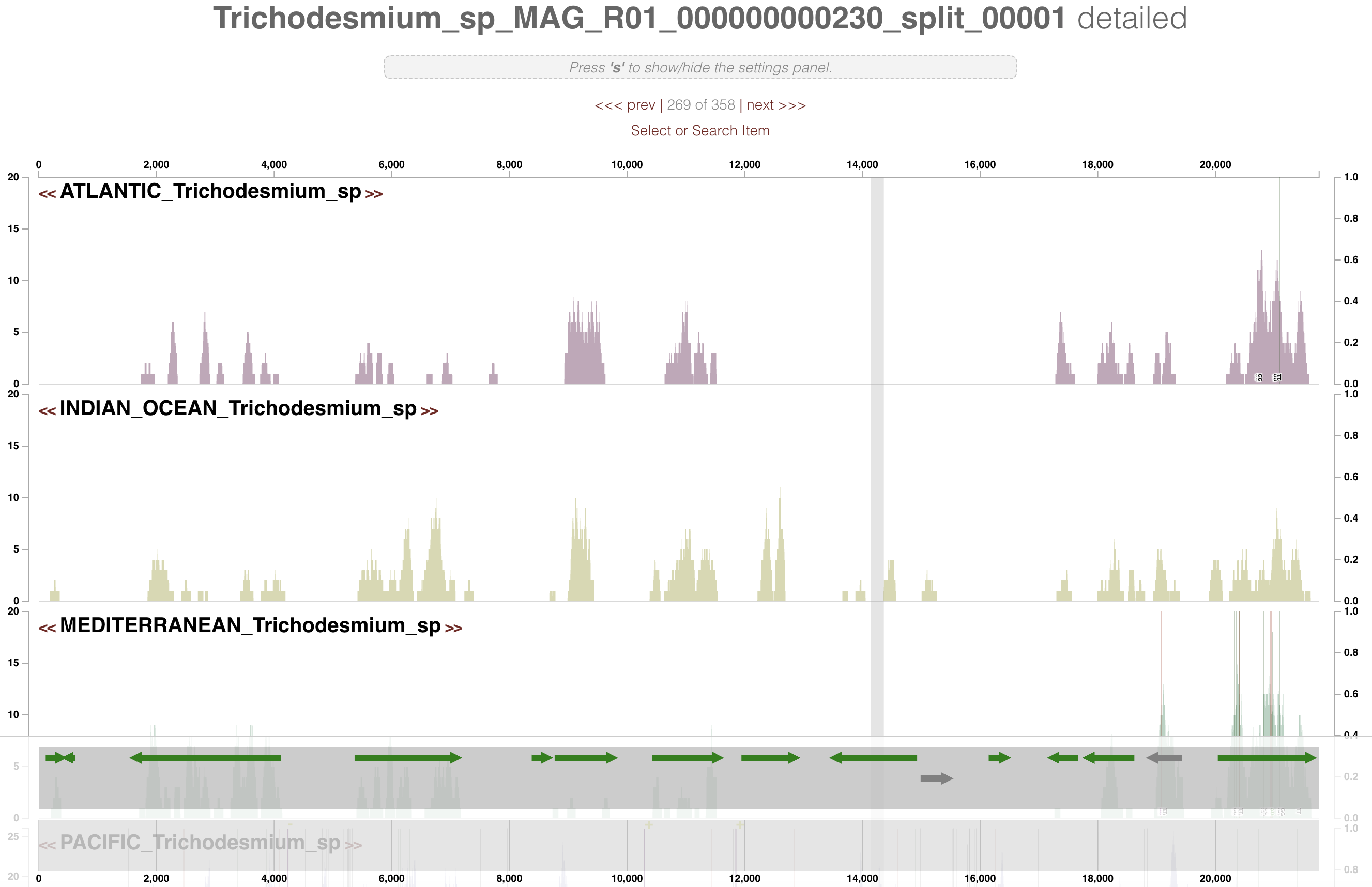
The top of the page indicates that we are looking at a split of the contig named Trichodesmium_sp_MAG_R01_000000000230, and each bar plot shows the detailed per-nucleotide coverage for one of the samples. If you click through the rest of the splits of this contig (using the ‘prev’ and ‘next’ buttons at the top until the page title shows a different contig name), you should see largely the same pattern: in PACIFIC, the contig sequence is thoroughly covered but with wavy coverage depth and plenty of SNVs; in the top three samples the reads map more sporadically, with INDIAN_OCEAN often yielding the most consistent coverage; and in RED_SEA there are mostly isolated read-pairs scattered across the contig. This tracks with the summarized data we saw before.
Note that we see a lot of SNVs in the PACIFIC layer, but that is largely because this is the only layer in which the coverage depth is consistently deep enough for anvi-profile to take note of sequence variants (by default, the required depth is 10x). There are likely many differences between mapped reads and the reference sequence in the other samples, but not enough coverage for us to confidently distinguish true variation from sequencing errors.
Here are a few of the other interesting things you might notice as you look through this contig:
- a small missing region in the
PACIFIClayer containing a transposase gene (insplit_00003) - a huge spike of read recruitment with plenty of SNVs in between a phage lysozyme and an unannotated gene, in the top 3 samples (also in
split_00003) - an operon containing nifH, nifD, nifK and other nif genes that is covered only in
PACIFICandINDIAN_OCEAN(insplit_00006) - a large region with hardly any coverage (even in
PACIFIC) containing glycosyl transferases and several other genes (insplit_00007). Could it have come from an integrated plasmid or phage?
Clearly, genome-level and even contig-level coverage statistics can obscure a lot of variation in read recruitment patterns, especially when mobile genetic elements are involved.
If you want to open any of these splits directly from the command line, you could use the dedicated program anvi-inspect. Here is an example that opens the split with the nif operon:
anvi-inspect -c ../Trichodesmium_sp-contigs.db \
            -p NON_COMPETITIVE/TRICHO_SP_MERGED/PROFILE.db \
            --split-name Trichodesmium_sp_MAG_R01_000000000230_split_00006
Non-competitive read recruitment (mapping many metagenomes to many genomes in individual FASTA files)
This section is very similar to the previous one, both conceptually and in practice. Feel free to skip it if you don’t have enough time (you could move directly to competitive read recruitment instead).
We’ve just finished a rough biogeography analysis of Trichodesmium sp., which is actually a T. erythraeum based on our taxonomy estimates in Chapter 1. What about the other Trichodesmium species – where are they found across the global oceans? To find out, we just need to repeat the same process, but using other genomes as our references. We will use one representative from each of the remaining Trichodesmium species, specifically these genomes:
MAG_Trichodesmium_thiebautii_IndianMAG_Candidatus_Trichodesmium_miruMAG_Candidatus_Trichodesmium_nobis
The T. miru and T. nobis MAGs were selected because they are the only representatives in our datapack of those species, and MAG_Trichodesmium_thiebautii_Indian was chosen because it is the most complete T. thiebautii genome we have (remember the genome completeness table from Chapter 1?).
We will stick with non-competitive read recruitment for now, meaning that each sample will be mapped to each genome independently. The consequence is that a given sequencing read could map to multiple of the genomes, as long as its sequence has a good match somewhere in each reference. That is, the genomes aren’t competing with each other to recruit reads. If there are multiple Trichodesmium species in one sample, the reads from regions that are similar across all these genomes (like ribosomal proteins or other shared genes) will all map repeatedly to each reference, even if that reference is a different Trichodesmium than the population the DNA originally came from. In other words, non-specific read recruitment can and will happen. But that is okay – non-specific mapping is a common occurrence since our mapping references will almost never contain the exact same set of populations in our metagenome samples, so we have to learn how to deal with it.
Let’s first extract our three genomes of interest and the paths to their contigs databases from the external genomes file in the parent directory:
for g in MAG_Trichodesmium_thiebautii_Indian MAG_Candidatus_Trichodesmium_miru MAG_Candidatus_Trichodesmium_nobis
do
  grep $g ../external-genomes.txt >> genomes_to_map.txt
done
This file will make the downstream work a bit easier.
To make things a bit cleaner, we’ll put the read recruitment and profiling commands into a BASH script and use variables to control which genome/sample pair we are mapping. Since you’ve finished the previous sections of this tutorial, you already know how to do all these steps (including working with loops and variables).
Exercise 1: Create a BASH script to do non-competitive read recruitment.
Your script should loop over the 3 selected representative genomes, extract their contig sequences, make Bowtie indexes out of each one, and then loop over all 5 metagenome samples to run the read mapping and profiling steps. At the end, it should merge all single-sample profiles for the same genome into one profile database. It is your choice if you want to take care of these steps using completely separate loops, or a couple of nested loops. Pro Tip: use the genomes_to_map.txt and samples.txt files to get paths to the files you need rather than hard-coding everything. Please name your script map_noncompetitive.sh for consistency with later tutorial commands. When you are ready to check your answer, click the Show/Hide box below.
Show/Hide Answer to Exercise 1: script for non-competitive mapping
Here is one possible solution:
#!/bin/bash
# a script to run non-competitive read recruitment

INPUT_GENOMES="genomes_to_map.txt"
INPUT_SAMPLES="samples.txt"
OUTPUT_DIR="NON_COMPETITIVE"

while read g db
do
  anvi-export-contigs -c $db -o ${g}.fa
  bowtie2-build ${g}.fa $g
  while read sample r1 r2
  do
    echo "Mapping $sample to $g"
    bowtie2 -x $g -1 $r1 -2 $r2 -S ${OUTPUT_DIR}/${sample}-${g}.sam
    samtools view -F 4 -bS ${OUTPUT_DIR}/${sample}-${g}.sam -o ${OUTPUT_DIR}/${sample}-${g}-RAW.bam
    samtools sort ${OUTPUT_DIR}/${sample}-${g}-RAW.bam -o ${OUTPUT_DIR}/${sample}-${g}.bam
    samtools index ${OUTPUT_DIR}/${sample}-${g}.bam
    rm ${OUTPUT_DIR}/${sample}-${g}.sam ${OUTPUT_DIR}/${sample}-${g}-RAW.bam
    anvi-profile -i ${OUTPUT_DIR}/${sample}-${g}.bam -c $db -o ${OUTPUT_DIR}/${sample}-${g}-PROFILE
  done < <(tail -n+2 samples.txt) # notice here that we don't skip the first sample row
  anvi-merge ${OUTPUT_DIR}/*-${g}-PROFILE/PROFILE.db -c $db -o ${OUTPUT_DIR}/${g}_MERGED
done < $INPUT_GENOMES
There is a copy of this script in your datapack, and if you want to use it (instead of your own script), you can copy it over to your working directory:
cp ../00_DATA/mapping/map_noncompetitive.sh .
Sounds like way too much for your laptop to handle? A script like this is fairly easy to run as a job on an HPC, in case you have access to one.
This script will take several minutes to run, because it processes each genome and each sample sequentially. If you are running this on a laptop, you should be prepared to leave it open and connected to power until it is done. If you are running this on an HPC, please make sure you are running it on a compute node and not a head node (you may need to send the command to your HPC’s job scheduler).
To run the script and direct all its output (including errors) into a log file:
# should take ~10 minutes to run
./map_noncompetitive.sh > noncompetitive.log 2>&1
If you are short on time (or computational resources) and you prefer not to run this script by yourself, you can access the final merged profiles saved in the datapack by following the instructions in the Show/Hide box below.
Show/Hide Copying over the merged profiles for visualization
Here is how to get our backup databases if you don’t want to run the read recruitment yourself:
cp -r ../00_DATA/mapping/BACKUP_PROFILES/MAG*_MERGED NON_COMPETITIVE/
Exercise 2: Visualize the non-competitive read recruitment results. After running the read recruitment script (or copying over the backup data), you should now have 4 merged profile databases, each paired with one of our Trichodesmium references. We’ve already looked at the data for Trichodesmium sp., but now is your chance to visualize one or more of the other 3 genomes’ results in the interactive interface. Consider the following questions: (1) In which sample(s) is the genome detected? (2) Is the entire genome observed in those samples? (3) What is the average coverage of the genome in those samples?
Show/Hide Answer to Exercise 2: non-competitive visualizations and interpretation
Assuming your script created merged profile databases in the NON_COMPETITIVE/ directory, here is a loop to visualize the results for each genome:
while read g db
do
  anvi-interactive -c $db -p NON_COMPETITIVE/${g}_MERGED/PROFILE.db --title $g
done < genomes_to_map.txt
If you look at the data without modifying anything in the interface, it looks like reads are mapping all over each reference. But with a few tweaks (focusing on detection and Q2Q3 coverage instead of the default mean coverage, setting some reasonable minimum and maximum values), you can get a bit closer to understanding the ‘true’ distribution of these genomes.
Here is how I interpreted the visualization for each genome:
- MAG_Trichodesmium_thiebautii_Indian: the only sample in which this genome is highly detected is
INDIAN_OCEAN. Some of its contigs are also detected inPACIFICandMEDITERRANEAN, but not all. On average, the genome seems to have a Q2Q3 coverage of ~3x inINDIAN_OCEAN, though there are a couple of contigs in which the mean coverage spikes to as high as ~56x, driven by individual genes (including a transposase) that are recruiting lots of reads - MAG_Candidatus_Trichodesmium_miru: this genome is detected in
ATLANTICwith a Q2Q3 coverage of ~4-5x, and partially detected inMEDITERRANEANandPACIFICwith somewhat less coverage. The coverage depth appears much less consistent in these two samples than inATLANTIC, and that combined with the large missing region suggests thatATLANTICis the only sample in which this organism is truly present (that is, it gathered non-specific read recruitment from a different Trichodesmium species inMEDITERRANEANandPACIFIC) - MAG_Candidatus_Trichodesmium_nobis: this genome is certainly detected in
MEDITERRANEAN, but only half of its contigs (or fewer) have decent detection scores in the other samples, and coverage depth is quite inconsistent in those other samples. It seems to be covered ~5x inMEDITERRANEAN.
Because I generated the datapack, I can let you in on a little secret – each of our metagenomes contains reads that map to exactly two of our genomes: the first is always Trichodesmium sp. and the second is always another MAG. The true genome-sample pairing is as follows:
MAG_Trichodesmium_thiebautii_Indianis present inINDIAN_OCEANMAG_Candidatus_Trichodesmium_miruis present inATLANTIC. Note that I also kept reads mapping to this genome in thePACIFICsample, but I believe these to be non-specificMAG_Candidatus_Trichodesmium_nobisis present inMEDITERRANEAN. Note that I also kept reads mapping to this genome in theRED_SEAsample, though these are either non-specific or Ca. T. nobis is in extremely low abundance there (analogous to the situation we saw earlier for Trichodesmium sp. in this sample)
So non-specific read recruitment really muddled the picture for us here. It made several contigs of T. thiebautii appear present in PACIFIC and MEDITERRANEAN, even though those reads were coming from different species. The Ca. T. miru genome recruited plenty of reads from Ca. T. nobis in the MEDITERRANEAN sample, and from whatever local Trichodesmium population belongs to PACIFIC, such that a large portion of its genome appeared covered in those samples. The same thing happened in the non-MEDITERRANEAN samples for Ca. T. nobis.
Regardless, with a bit of care, we were able to push past the non-specific read recruitment signal and identify the sample in which each genome was truly present.
Here is one of the visualizations, for Ca. T. miru, in case you want to compare it to the competitive read recruitment picture later:
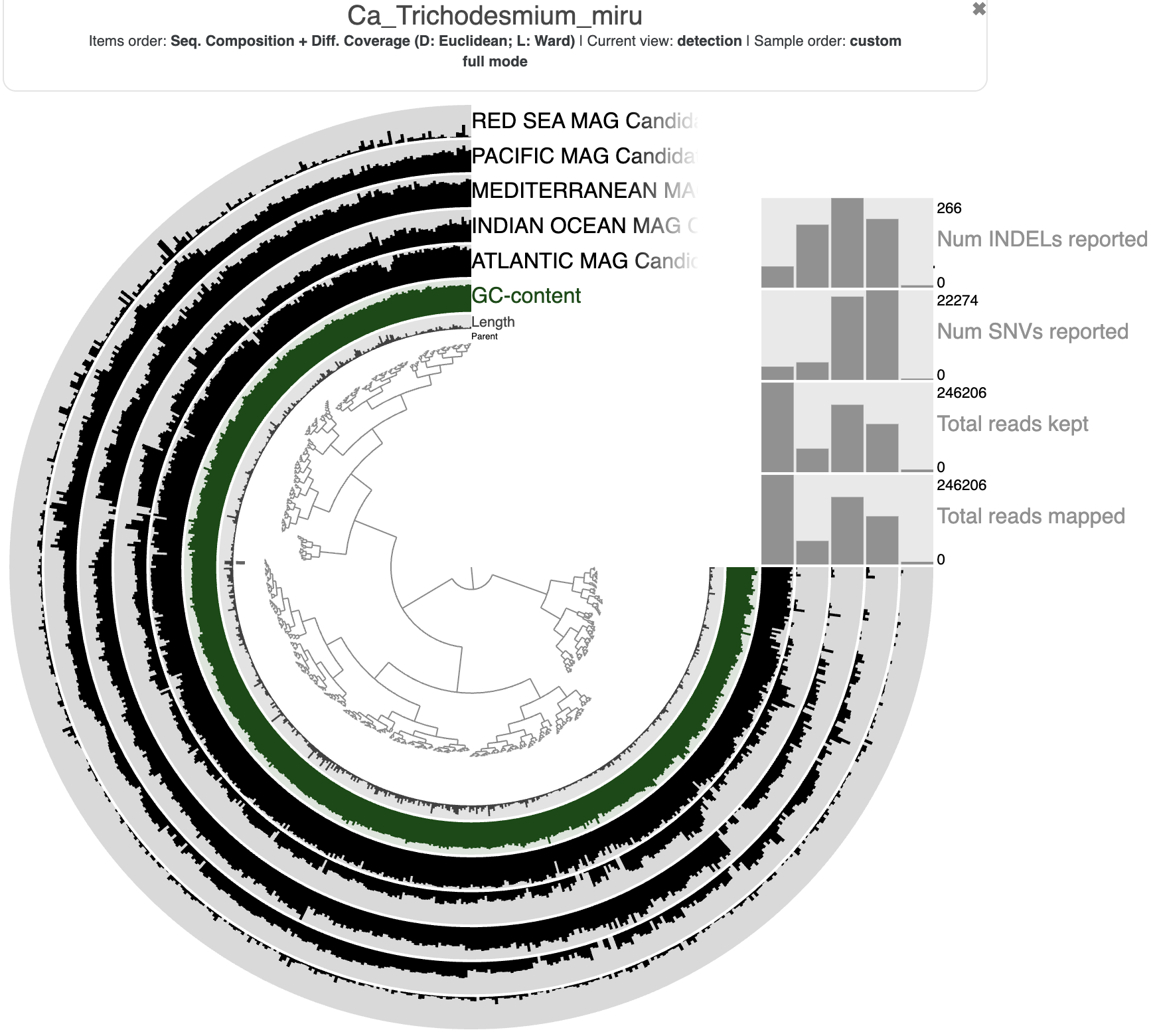
What you should take away from this section is that even though non-competitive read recruitment yields plenty of non-specific signal, we can often manage to distinguish between genome presence and absence anyway. That said, the picture will be much cleaner when we do competitive read recruitment in the next section.
Clean-up
Feel free to keep the merged profile databases in case you want to go through the data again interactively later (particularly to compare with the competitive read recruitment results). But we don’t need the BAM files or the single-sample profile dbs anymore. We’re also done with the individual Bowtie indices for each genome. Let’s clean these up from our working and output directories:
rm -r NON_COMPETITIVE/*.bam NON_COMPETITIVE/*.bai NON_COMPETITIVE/*-PROFILE/ *.bt2
Competitive read recruitment (mapping many metagenomes to many genomes in ONE combined FASTA file)
Show/Hide Did you skip non-competitive read recruitment? Click here for data preparation steps.
If you haven’t run the above section(s) on non-competitive read recruitment, then you should follow these steps to obtain a few of the files we will need.
# get a file of genomes and their database paths
rm -f genomes_to_map.txt
for g in MAG_Trichodesmium_thiebautii_Indian MAG_Candidatus_Trichodesmium_miru MAG_Candidatus_Trichodesmium_nobis Trichodesmium_sp
do
  grep $g ../external-genomes.txt >> genomes_to_map.txt
done
# export contig sequences from each genome
while read g db
do
  anvi-export-contigs -c $db -o ${g}.fa
done < genomes_to_map.txt
# make a collection-txt for Trichodesmium sp.
grep '>' Trichodesmium_sp.fa | sed 's/>//g' > contigs
cut -d '_' -f 1-4 contigs > genome
paste contigs genome > Trichodesmium_sp_collection.txt
rm contigs genome
You should see four FASTA files in your working directory:
$ ls *.fa
MAG_Candidatus_Trichodesmium_miru.fa  MAG_Candidatus_Trichodesmium_nobis.fa  MAG_Trichodesmium_thiebautii_Indian.fa  Trichodesmium_sp.fa
We are now going to do competitive read recruitment, meaning that we’ll map our metagenome samples to all four genomes at once. Each sequencing read will therefore map to the genome that it best matches to, even if it is technically similar enough to match a sequence in multiple genomes. This strategy can greatly reduce the influence of non-specific read recruitment in our results. Another advantage is that it will be a little bit faster, because we only have a single reference to map to instead of four individual references.
The first step is to combine all four of our genomes into one reference FASTA file:
cat *.fa > COMBINED.fa
An important caveat to this is that all of the contig sequences can be uniquely matched to their original genome, via the prefixes in their contig headers. For instance, all the contig names belonging to MAG_Candidatus_Trichodesmium_miru start with the string TARA_AOS_82_MAG_00025. This will become important later, when we want to separate the four genomes again in our results.
Let’s run all the steps of read recruitment, but on this combined FASTA file. We’ll use a script to do it (and I won’t make you write it yourself this time unless you really want to wink wink).
Here is the script. It starts by building a Bowtie 2 index and a contigs database for the combined set of genomes, and then loops over each metagenome to run all the mapping steps. At the end, it merges the single profiles together. All the mapping output is created in the directory called COMPETITIVE to keep it separate from our earlier work:
#!/bin/bash
# a script to run competitive read recruitment

INPUT_GENOMES_FA="COMBINED.fa"
INPUT_SAMPLES="samples.txt"
OUTPUT_DIR="COMPETITIVE"

g="COMBINED"
db="${g}.db"

mkdir -p $OUTPUT_DIR

bowtie2-build ${g}.fa $g
anvi-gen-contigs-database -f $INPUT_GENOMES_FA -o $db

while read sample r1 r2
do
    echo "Mapping $sample to $g"
    bowtie2 -x $g -1 $r1 -2 $r2 -S ${OUTPUT_DIR}/${sample}-${g}.sam
    samtools view -F 4 -bS ${OUTPUT_DIR}/${sample}-${g}.sam -o ${OUTPUT_DIR}/${sample}-${g}-RAW.bam
    samtools sort ${OUTPUT_DIR}/${sample}-${g}-RAW.bam -o ${OUTPUT_DIR}/${sample}-${g}.bam
    samtools index ${OUTPUT_DIR}/${sample}-${g}.bam
    rm ${OUTPUT_DIR}/${sample}-${g}.sam ${OUTPUT_DIR}/${sample}-${g}-RAW.bam
    anvi-profile -i ${OUTPUT_DIR}/${sample}-${g}.bam -c $db -o ${OUTPUT_DIR}/${sample}-${g}-PROFILE
done < <(tail -n+2 samples.txt)

anvi-merge ${OUTPUT_DIR}/*-${g}-PROFILE/PROFILE.db -c $db -o ${OUTPUT_DIR}/${g}_MERGED
For convenience, you can copy the script over from the data dir before running it:
cp ../00_DATA/mapping/map_competitive.sh .

# should take ~8 minutes to run
./map_competitive.sh > competitive.log 2>&1
Now that you understand the different steps required for read recruitment, there is a much better way to actually run all those steps, and that is to use workflows. Anvi’o has a built-in snakemake workflow for metagenomics which can be run in ‘references mode’ to perform read recruitment from multiple samples to one or more references, with the option to go all the way to merged profile databases. If you want to learn how to do this with your own data, check out Meren’s tutorial on competitive read recruitment or Florian’s more general tutorial on workflows.
Once the script is done, you can visualize it as follows:
anvi-interactive -c COMBINED.db \
        -p COMPETITIVE/COMBINED_MERGED/PROFILE.db \
        --title Combined_Genomes
But there is one problem – you can’t tell which contig belongs to which genome in the display. We need to import a collection of bins describing our genomes first. Stop the interface server, and then run the following commands to make a collection-txt file describing, for each contig, which genome it belongs to:
for fa in MAG_*.fa
do
  genome="${fa%.*}"
  while read contig
  do
    echo -e "$contig\t$genome" >> COMBINED_collection.txt
  done < <(grep '>' $fa | sed 's/>//g')
done
cat Trichodesmium_sp_collection.txt >> COMBINED_collection.txt
The outer loop here goes through each FASTA file starting with MAG_, and extracts the name of the genome by removing the .fa extension of the file name. The inner loop then goes over each contig name in the FASTA file (identified by searching for the ‘>’ characters and then removing those characters) and writes it to the collection file along with the genome name. Afterwards, we add in the Trichodesmium sp. contigs from the Trichodesmium_sp_collection.txt file that we already created.
We can import this collection into our profile database. You can name it ‘default’ so that it shows up automatically when you open the interface:
anvi-import-collection -p COMPETITIVE/COMBINED_MERGED/PROFILE.db \
        -c COMBINED.db \
        -C default \
        --contigs-mode \
        COMBINED_collection.txt
Afterwards, opening the interface (same command as before) should show you a clear story:
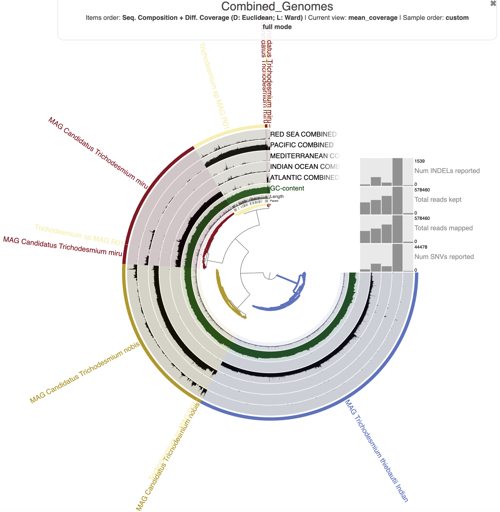
First, the contigs are organized according to their sequence composition and differential coverage, which means that contigs from the same genome largely come together. There are a few exceptions because these are closely-related genomes. In particular, they have very similar sequence composition – if you change the organization to sequence composition, you should see that all the genomes get mixed up. Organizing the contigs by differential coverage alone does a much better job at keeping the original genomes distinct.
Second, you should see that each genome has clean read recruitment from one sample, with limited signal from all other samples. This becomes especially clear if you switch the data view to Q2Q3 coverage. You might recall that the displays from non-competitive read recruitment were much messier – that was due to non-specific read recruitment that has been largely eliminated by using the competitive mapping strategy.
So, which genome is found in which sample(s)? Take a look at the detection data:
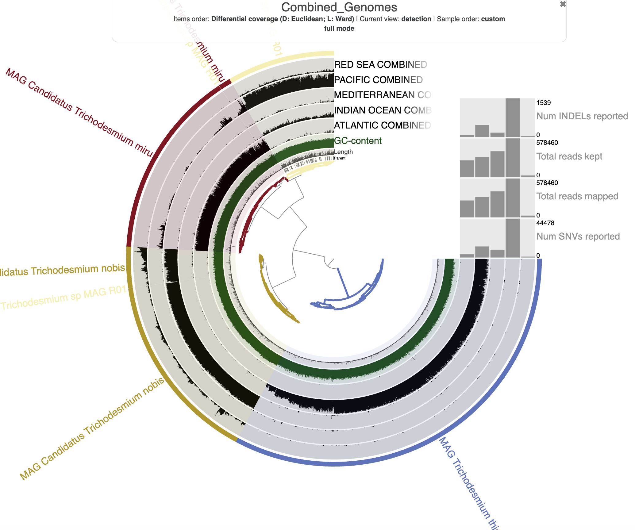
If you want to use our visualization settings, feel free to run
anvi-import-state -p COMPETITIVE/COMBINED_MERGED/PROFILE.db -s ../00_DATA/mapping/combined_state.json -n tutorial
and then re-open the interface and load the state called ‘tutorial’.
As we saw before, Trichodesmium sp. is found in PACIFIC, thiebautii is found in INDIAN_OCEAN, miru is found in ATLANTIC and nobis is found in MEDITERRANEAN. It is also debatable whether nobis and Trichodesmium sp. are found in very low abundance in RED_SEA and/or INDIAN_OCEAN, respectively, given the roughly even detection signal across their genomes in these samples.
We can summarize this quantitatively by running anvi-profile-blitz on the BAM files with our collection:
# then run the blitz
anvi-profile-blitz -C COMBINED_collection.txt \
                -c COMBINED.db \
                -o COMPETITIVE/combined_genome_stats.txt \
                COMPETITIVE/*-COMBINED.bam
In the output table, we can see that the detection and dis_cov scores recapitulate what we’ve seen in the interface. Distribution of coverage seems to indicate that Trichodesmium sp. is indeed found in INDIAN_OCEAN, but we are a bit less confident about its presence in the RED_SEA than we were earlier using non-competitive read recruitment.
bin |
sample |
length |
gc_content |
num_mapped_reads |
detection |
mean_cov |
q2q3_cov |
median_cov |
min_cov |
max_cov |
std_cov |
num_windows |
prop_windows_covered |
prop_cov_within_foldrange |
dis_cov |
|---|---|---|---|---|---|---|---|---|---|---|---|---|---|---|---|
| MAG_Candidatus_Trichodesmium_miru | ATLANTIC-COMBINED | 5425804 | 0.351 | 243910 | 0.9102 | 4.514 | 4.037 | 4.0 | 0 | 370 | 4.092 | 5426 | 0.9952 | 0.7839 | 0.8895 |
| MAG_Candidatus_Trichodesmium_nobis | ATLANTIC-COMBINED | 6101640 | 0.359 | 142 | 0.001913 | 0.002294 | 0.0 | 0.0 | 0 | 5 | 0.05761 | 6102 | 0.01868 | 0.9675 | 0.4931 |
| MAG_Trichodesmium_thiebautii_Indian | ATLANTIC-COMBINED | 6834732 | 0.353 | 80 | 0.0008925 | 0.00116 | 0.0 | 0.0 | 0 | 7 | 0.04578 | 6835 | 0.008632 | 0.9449 | 0.4768 |
| Trichodesmium_sp_MAG_R01 | ATLANTIC-COMBINED | 6640707 | 0.34 | 7708 | 0.0348 | 0.1162 | 0.0 | 0.0 | 0 | 97 | 1.098 | 6641 | 0.1316 | 0.8119 | 0.4718 |
| MAG_Candidatus_Trichodesmium_miru | INDIAN_OCEAN-COMBINED | 5425804 | 0.351 | 199 | 0.00295 | 0.003663 | 0.0 | 0.0 | 0 | 8 | 0.07848 | 5426 | 0.02893 | 0.9536 | 0.4913 |
| MAG_Candidatus_Trichodesmium_nobis | INDIAN_OCEAN-COMBINED | 6101640 | 0.359 | 460 | 0.005219 | 0.00752 | 0.0 | 0.0 | 0 | 11 | 0.1355 | 6102 | 0.04769 | 0.9232 | 0.4854 |
| MAG_Trichodesmium_thiebautii_Indian | INDIAN_OCEAN-COMBINED | 6834732 | 0.353 | 271890 | 0.8608 | 4.001 | 3.33 | 3.0 | 0 | 541 | 6.094 | 6835 | 0.9873 | 0.793 | 0.8901 |
| Trichodesmium_sp_MAG_R01 | INDIAN_OCEAN-COMBINED | 6640707 | 0.34 | 28857 | 0.1814 | 0.4366 | 0.0 | 0.0 | 0 | 181 | 2.321 | 6641 | 0.6615 | 0.7981 | 0.7298 |
| MAG_Candidatus_Trichodesmium_miru | MEDITERRANEAN-COMBINED | 5425804 | 0.351 | 507 | 0.004506 | 0.009031 | 0.0 | 0.0 | 0 | 52 | 0.2778 | 5426 | 0.04055 | 0.8627 | 0.4516 |
| MAG_Candidatus_Trichodesmium_nobis | MEDITERRANEAN-COMBINED | 6101640 | 0.359 | 371864 | 0.926 | 6.024 | 5.037 | 5.0 | 0 | 6392 | 22.12 | 6102 | 1.0 | 0.6453 | 0.8226 |
| MAG_Trichodesmium_thiebautii_Indian | MEDITERRANEAN-COMBINED | 6834732 | 0.353 | 446 | 0.003602 | 0.006275 | 0.0 | 0.0 | 0 | 51 | 0.2064 | 6835 | 0.03277 | 0.8797 | 0.4562 |
| Trichodesmium_sp_MAG_R01 | MEDITERRANEAN-COMBINED | 6640707 | 0.34 | 13736 | 0.03972 | 0.1964 | 0.0 | 0.0 | 0 | 728 | 2.918 | 6641 | 0.1589 | 0.7673 | 0.4631 |
| MAG_Candidatus_Trichodesmium_miru | PACIFIC-COMBINED | 5425804 | 0.351 | 21182 | 0.07811 | 0.3909 | 0.0 | 0.0 | 0 | 817 | 6.264 | 5426 | 0.2757 | 0.7385 | 0.5071 |
| MAG_Candidatus_Trichodesmium_nobis | PACIFIC-COMBINED | 6101640 | 0.359 | 254 | 0.00233 | 0.004154 | 0.0 | 0.0 | 0 | 14 | 0.1312 | 6102 | 0.0218 | 0.8806 | 0.4512 |
| MAG_Trichodesmium_thiebautii_Indian | PACIFIC-COMBINED | 6834732 | 0.353 | 635 | 0.003817 | 0.009235 | 0.0 | 0.0 | 0 | 63 | 0.3296 | 6835 | 0.03497 | 0.8278 | 0.4314 |
| Trichodesmium_sp_MAG_R01 | PACIFIC-COMBINED | 6640707 | 0.34 | 556389 | 0.9059 | 8.42 | 7.948 | 8.0 | 0 | 404 | 7.477 | 6641 | 0.9846 | 0.7625 | 0.8735 |
| MAG_Candidatus_Trichodesmium_miru | RED_SEA-COMBINED | 5425804 | 0.351 | 56 | 0.0007713 | 0.0009547 | 0.0 | 0.0 | 0 | 6 | 0.04016 | 5426 | 0.007741 | 0.967 | 0.4874 |
| MAG_Candidatus_Trichodesmium_nobis | RED_SEA-COMBINED | 6101640 | 0.359 | 16589 | 0.1142 | 0.2599 | 0.0 | 0.0 | 0 | 1879 | 6.795 | 6102 | 0.4595 | 0.8227 | 0.6411 |
| MAG_Trichodesmium_thiebautii_Indian | RED_SEA-COMBINED | 6834732 | 0.353 | 292 | 0.00284 | 0.004045 | 0.0 | 0.0 | 0 | 37 | 0.1337 | 6835 | 0.02955 | 0.9381 | 0.4838 |
| Trichodesmium_sp_MAG_R01 | RED_SEA-COMBINED | 6640707 | 0.34 | 10237 | 0.08158 | 0.154 | 0.0 | 0.0 | 0 | 53 | 0.8277 | 6641 | 0.3914 | 0.8527 | 0.622 |
Conclusions? If you want cleaner read recruitment results, go with a competitive mapping strategy. If you can’t do that, then you will need to be a bit more stringent when deciding on genome presence-absence in order to account for the influence of non-specific read recruitment.
Clean-up
Let’s get rid of the BAM files, indexes, and single profiles from this section:
rm -r COMPETITIVE/*.bam COMPETITIVE/*.bai COMPETITIVE/*-COMBINED-PROFILE *.bt2
What we’ve learned
The biggest take-away from this chapter is hopefully an awareness of non-specific read recruitment and how it influences read mapping results. But we’ve also learned:
- that we can decide on genome presence-absence by looking at summary statistics like detection and distribution of coverage
- that these summary statistics cover up a lot of variation in the mapping data. Individual genes or longer regions of your reference can be missing entirely from the local version of your reference population, and at a finer scale, the local population can have many SNVs or indels relative to the reference
Don’t forget to go back to the parent directory before you move on to the next tutorial section:
cd ..
Congrats!
This is currently the last chapter of the tutorial. Well done! We hope it was useful for you.
If you want to go back to the main page of the tutorial, click here.
If you have any questions about this exercise, or have ideas to make it better, please feel free to get in touch with the anvi’o community through our Discord server: