An anvi'o tutorial with Trichodesmium genomes


Table of Contents
- A story of nitrogen fixation (or not) in Trichodesmium
- Downloading the datapack
- Activating anvi’o
- Genomics
- Download and reformat the genome
- Generate a contigs database
- Annotate single-copy core genes and Ribosomal RNAs
- Estimate completeness and redundancy
- Estimate SCG taxonomy
- Functional annotations
- Working with multiple genomes
- Working with one (or more) metagenomes
- Pangenomics
- Genome storage
- Pangenome analysis
- Interactive pangenomics display
- Inspect gene clusters
- Bin and summarize a pangenome
- Search for functional annotations
- Additional genome information
- Metabolism
Summary
The purpose of this tutorial is to learn how to use the set of integrated ‘omics tools in anvi’o to make sense of a few Trichodesmium genomes. Here is a list of topics that are covered in this tutorial:
- Create contigs databases and run functional annotation programs.
- Estimate taxonomy and completion/redundancy across multiple genomes.
- Generate a pangenome of closely related Trichodesmium genomes.
- Study metabolism by predicting metabolic pathway completeness and metabolic interactions.
If you have any questions about this exercise, or have ideas to make it better, please feel free to get in touch with the anvi’o community through our Discord server:

To reproduce this exercise with your own dataset, you should first follow the instructions here to install anvi’o.
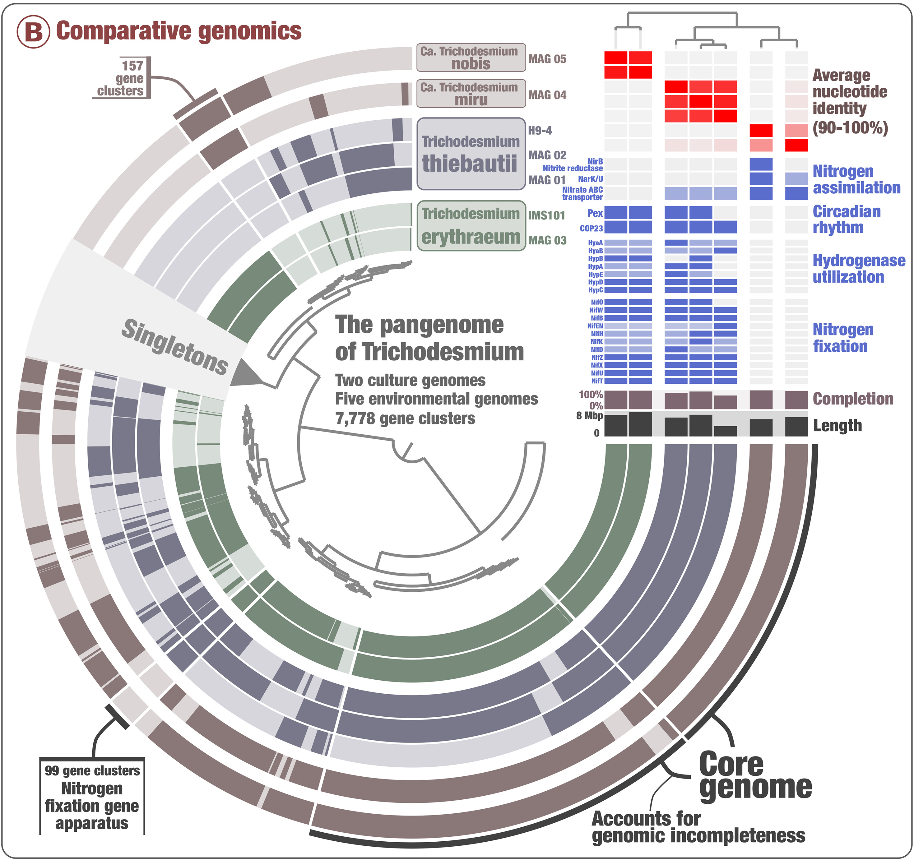
A story of nitrogen fixation (or not) in Trichodesmium
This tutorial will largely recapitulate a story from the following paper, published by Tom Delmont in 2021:
- Expanded the understanding of the ecological roles and diversity of Trichodesmium.
- Challenged long-held assumptions about nitrogen fixation in marine cyanobacteria.
As a little preview, the essence of the story is this: Trichodesmium species are well-known cyanobacterial nitrogen fixers (‘diazotrophs’) in the global oceans, but – surprise – it turns out that not all of them can do nitrogen fixation. Tom used a combination of pangenomics, phylogenomics, and clever read recruitment analyses on a set of MAGs and reference genomes to demonstrate that two new (candidate) Trichodesmium species, Candidatus T. miru and Candidatus T. nobis, are nondiazotrophic.
We will use a variety of anvi’o programs to investigate the same genomes and characterize their nitrogen-fixing capabilities, to demonstrate how you, too, could discover cool microbial ecology stories like this one.
Downloading the datapack
In your terminal, choose a working directory for this tutorial and use the following code to download the dataset:
curl -L https://figshare.com/ndownloader/files/58678165\
     -H "User-Agent: Chrome/115.0.0.0" \
     -o trichodesmium_tutorial.tar.gz
Then unpack it, and go into the datapack directory:
tar -zxvf trichodesmium_tutorial.tar.gz
cd trichodesmium_tutorial
At this point, if you check the datapack contents in your terminal with ls, this is what you should be seeing:
$ ls
00_DATA

$ ls 00_DATA/
associate_dbs             fasta                     metabolism_state.json     module_info.txt           nitrogen_heatmap.json     pan_state.json
contigs                   genome-pairs.txt          metagenome                modules                   nitrogen_step_copies.json
Inside the 00_DATA folder, there are several files that will be useful for various parts of this tutorial. We will start from the seven Trichodesmium genomes stored in the fasta directory. Some are metagenome-assembled genomes (MAGs) binned from the TARA Ocean metagenomic dataset, and others are reference genomes taken from NCBI RefSeq.
Activating anvi’o
Before you start, don’t forget to activate your anvi’o environment:
We use the development version of anvi’o here, but you could also use a stable release of anvi’o if that is what you have installed. Any stable release starting from v9 or later will include all of the programs covered in this tutorial. If you try an earlier release, you may see “command not found” errors for some of the commands.
conda activate anvio-dev
Genomics
To introduce you into the anvi’o-verse, we will run some basic genomics analysis on a single genome. In this case, we will download a known Trichodesmium genome from NCBI to add to our collection. We will learn how to:
- reformat a FASTA file
- generate a contigs-db
- annotate gene calls with single-copy core genes and functions
- estimate the taxonomy and completeness/redundancy of the genome
- get data out of the database and into parseable text files
Let’s get started.
Download and reformat the genome
We will supplement our set of Trichodesmium genomes with this Trichodesmium MAG from NCBI. It is labeled as Trichodesmium sp. MAG_R01, so we don’t know exactly what species of Trichodesmium this is (yet). The MAG was generated by researchers at the Hebrew University of Jerusalem from a Red Sea metagenome, and it is of scaffold-level quality.
To download the genome, we will use the command curl:
curl https://ftp.ncbi.nlm.nih.gov/genomes/all/GCA/023/356/555/GCA_023356555.1_ASM2335655v1/GCA_023356555.1_ASM2335655v1_genomic.fna.gz -o GCA_023356555.1_ASM2335655v1_genomic.fna.gz
gunzip GCA_023356555.1_ASM2335655v1_genomic.fna.gz
Now we have one of the most fundamental files that everyone will have to interact with: a FASTA file. We can already check the number of contigs by counting the number of > characters, which appears once per sequence. We can use the command grep for that:
$ grep -c '>' GCA_023356555.1_ASM2335655v1_genomic.fna
269
That’s a lot of sequences, or in this case: a lot of contigs. That is already telling us a few things about this genome: it is not a singular contig representing a complete and circular genome. Let’s have a look at the contig headers:
grep '>' GCA_023356555.1_ASM2335655v1_genomic.fna
As you can see, the headers are rather complex, with a lot of information. Unfortunately, these headers are going to be problematic for downstream analysis, particularly because they include non-alphanumeric characters like spaces, dots, pipe (|) and whatnot. And anvi’o knows you would be in trouble if you start working this these headers. Just for fun, you can try to run anvi-gen-contigs-database (we will cover what it does very soon), and you will see an error:
anvi-gen-contigs-database -f GCA_023356555.1_ASM2335655v1_genomic.fna \
                          -o CONTIGS.db \
                          -T 2
Config Error: At least one of the deflines in your FASTA File does not comply with the 'simple
              deflines' requirement of anvi'o. You can either use the script `anvi-script-
              reformat-fasta` to take care of this issue, or read this section in the tutorial
              to understand the reason behind this requirement (anvi'o is very upset for
              making you do this): http://merenlab.org/2016/06/22/anvio-tutorial-v2/#take-a-
              look-at-your-fasta-file
We can use anvi-script-reformat-fasta to simplify the FASTA’s headers with the flag --simplify-names. This command can (optionally) generate a summary report, which is a two column file matching the new and old names of each sequence in the FASTA file. While we are using this command, we can use it to include a specific prefix in the renamed headers with the flag --prefix and filter out short contigs (in this example, smaller than 500 bp) with the flag -l.
anvi-script-reformat-fasta GCA_023356555.1_ASM2335655v1_genomic.fna \
                           -o Trichodesmium_sp.fa \
                           --simplify-names \
                           --prefix Trichodesmium_sp_MAG_R01 \
                           -r Trichodesmium_sp_reformat_report.txt \
                           -l 500 \
                           --seq-type NT
You can use this command to further filter your FASTA file: check the options with the online help page, or by using the flag --help in the terminal.
Generate a contigs database
The contigs-db is a central database in the anvi’o ecosystem. It essentially stores all information about a given set of (nucleotide) sequences from a FASTA file. To make a contigs-db from our reformatted FASTA, you can use the command anvi-gen-contigs-database:
Numerous anvi’o commands can make use of multithreading to speed up computing time. You can either use the flag -T or --num-threads. Check the help page of a command, or use --help to check if multithreading is available.
anvi-gen-contigs-database -f Trichodesmium_sp.fa \
                          -o Trichodesmium_sp-contigs.db \
                          -T 2
A few things happen when you generate a contigs-db. First, all DNA sequences are stored in that databases. You can retrieve the sequences in FASTA format by using the command anvi-export-contigs. Second, anvi’o uses pyrodigal-gv to identify open-reading frames (also referred to as ‘gene calls’). Pyrodigal-gv is a python implementation of Prodigal with some additional metagenomic models for giant viruses and viruses with alternative genetic codes (see Camargo et al.).
In addition to identifying open-reading frames, anvi’o will predict the amino acid sequence associated with each gene call and store it in that newly made database. If you need to get this information out of the database, you can use the command anvi-export-gene-calls to export the gene calls, and the amino acid sequence for each open-reading frame identified by pyrodigal-gv.
The command anvi-gen-contigs-database also computes the tetra-nucleotide frequency for each contig. To learn more about what it is, check the vocabulary page about tetra-nucleotide frequency.
Annotate single-copy core genes and Ribosomal RNAs
There is a command called anvi-run-hmms, which let you use Hidden Markov Models (HMMs) to annotate the genes in a contigs-db and store that annotation directly back into the database.
The anvi’o codebase comes with an integrated set of default HMM sources. They include models for 6 Ribosomal RNAs (16S, 23S, 5S, 18S, 28S, and 12S). They also include three sets of single-copy core genes, named Bacteria_71, Archaea_76 and Protista_83. The first two, Bacteria_71 and Archaea_76, are collections of bacterial and archaeal single-copy core genes (SCGs) curated from Mike Lee’s SCG collections first released in GToTree, which is an easy-to-use phylogenomics workflow. Protista_83 is a curated collection of BUSCO SCGs made by Tom Delmont. These sets of HMMs are used in anvi’o to compute the estimated completeness and redundancy of a genome.
To annotate our contigs-db with these HHMs, we can simply run anvi-run-hmms like this:
anvi-run-hmms -c Trichodesmium_sp-contigs.db -T 4
There is an optional flag --also-scan-trnas which uses the program tRNAScan-SE to identify and store information about tRNAs found in your genome. You can also use the command anvi-scan-trnas at any time.
Now is probably a good time to use the command anvi-db-info, which shows you basic information about any anvi’o database:
anvi-db-info Trichodesmium_sp-contigs.db
With this command, you can see which HMMs were already run on that database, but also some basic information like the number of contigs, number of genes called by pyrodigal-gv, and more:
DB Info (no touch)
===============================================
Database Path ................................: Trichodesmium_sp-contigs.db
description ..................................: [Not found, but it's OK]
db_type ......................................: contigs (variant: unknown)
version ......................................: 24


DB Info (no touch also)
===============================================
project_name .................................: Trichodesmium_sp
contigs_db_hash ..............................: hash0d1122fb
split_length .................................: 20000
kmer_size ....................................: 4
num_contigs ..................................: 269
total_length .................................: 6640707
num_splits ...................................: 358
gene_level_taxonomy_source ...................: None
genes_are_called .............................: 1
external_gene_calls ..........................: 0
external_gene_amino_acid_seqs ................: 0
skip_predict_frame ...........................: 0
splits_consider_gene_calls ...................: 1
trna_taxonomy_was_run ........................: 0
trna_taxonomy_database_version ...............: None
reaction_network_ko_annotations_hash .........: None
reaction_network_kegg_database_release .......: None
reaction_network_modelseed_database_sha ......: None
reaction_network_consensus_threshold .........: None
reaction_network_discard_ties ................: None
creation_date ................................: 1760017061.92556
scg_taxonomy_was_run .........................: 1
scg_taxonomy_database_version ................: GTDB: v214.1; Anvi'o: v1
gene_function_sources ........................: COG24_FUNCTION,COG24_PATHWAY,COG24_CATEGORY,KOfam,KEGG_BRITE,KEGG_Class,KEGG_Module
modules_db_hash ..............................: 66e53d49e65a

* Please remember that it is never a good idea to change these values. But in some
  cases it may be absolutely necessary to update something here, and a
  programmer may ask you to run this program and do it. But even then, you
  should be extremely careful.


AVAILABLE GENE CALLERS
===============================================
* 'pyrodigal-gv' (4,820 gene calls)


AVAILABLE FUNCTIONAL ANNOTATION SOURCES
===============================================
* No functional annotations found in this contigs database :/


AVAILABLE HMM SOURCES
===============================================
* 'Archaea_76' (76 models with 34 hits)
* 'Bacteria_71' (71 models with 72 hits)
* 'Protista_83' (83 models with 38 hits)
* 'Ribosomal_RNA_12S' (1 model with 0 hits)
* 'Ribosomal_RNA_16S' (3 models with 0 hits)
* 'Ribosomal_RNA_18S' (1 model with 0 hits)
* 'Ribosomal_RNA_23S' (2 models with 0 hits)
* 'Ribosomal_RNA_28S' (1 model with 0 hits)
* 'Ribosomal_RNA_5S' (5 models with 0 hits)
General summary and metrics
To go one step further than the output generated by anvi-db-info, we can use the command anvi-display-contigs-stats. It allows you to visualize (and export) basic information about one or multiple contigs databases.
anvi-display-contigs-stats Trichodesmium_sp-contigs.db
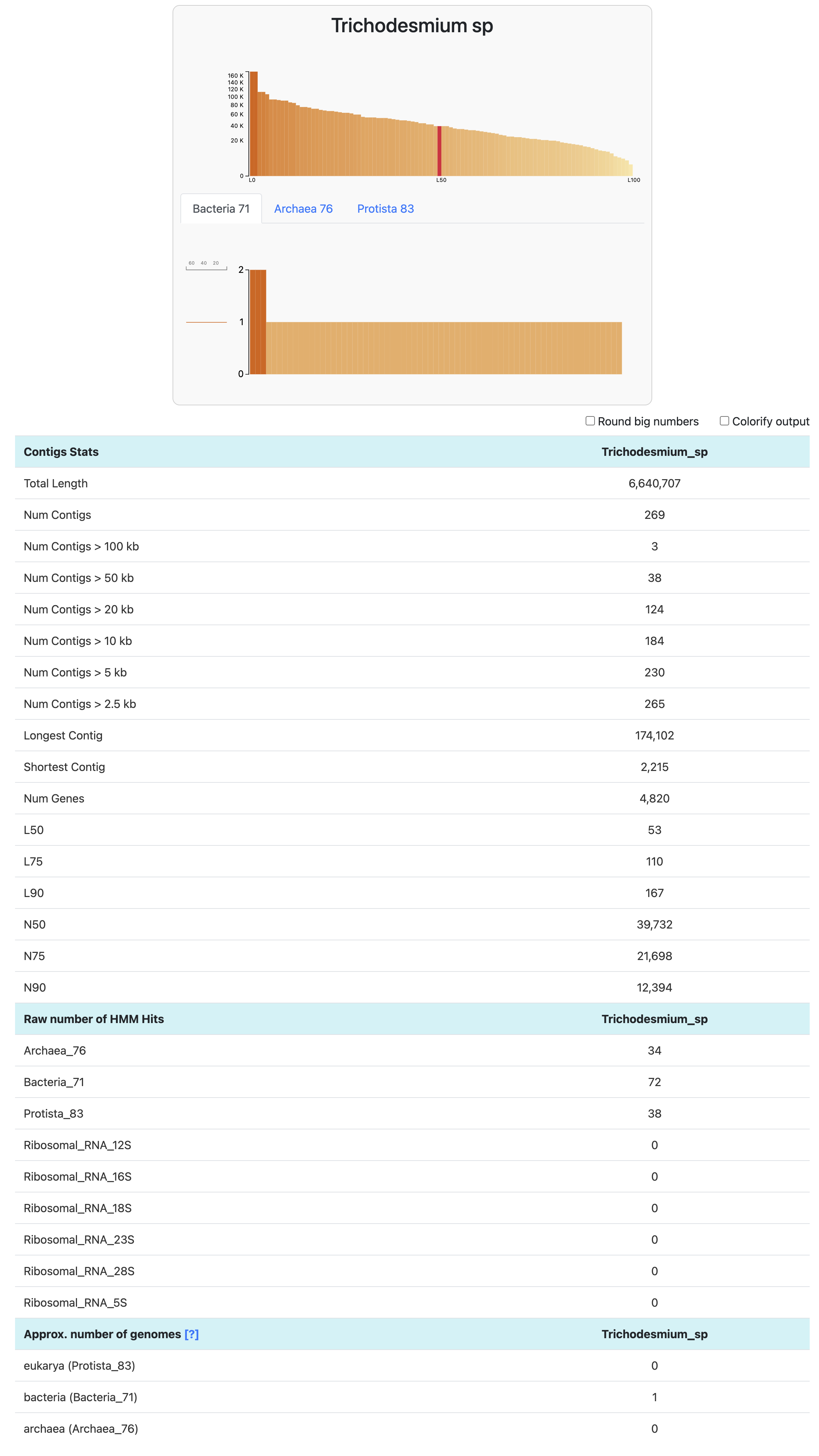
The approximate number of genomes is an estimate based on the frequency of each single-copy core gene (more info here). It is mostly useful in a metagenomics context, where you expect multiple microbial populations to be included in your set of contigs. This estimate is based on the mode (or most frequently occurring number) of single-copy core genes. Here, we know we generated a contigs-db with a single genome, hence the expected number of genomes = 1 bacteria. GOOD.
You can also export the information displayed on your browser by running anvi-display-contigs-stats with the flag --output-file or -o. Anvi’o will then write a TAB-delimited file with the above values. And if you don’t want the browser page to open at all, you can also use the flag --report-as-text.
anvi-display-contigs-stats Trichodesmium_sp-contigs.db --report-as-text -o Trichodesmium_sp-contigs-stats.txt
Estimate completeness and redundancy
We can use the set of single-copy core genes (SCGs) to estimate the completeness of a genome. The rational is pretty simple: we expect a set of genes to be systematically present in all genomes only once. So if we find all these genes, we estimate that the genome is complete (100%). We can also report how many SCGs are found in multiple copies, which we refer to as SCG ‘redundancy’.
Why redundancy and not contamination? The presence of multiple copies of SCGs could be indicative of contamination in your genome - i.e., the potential presence of more than one population - but microbial genomes have a bad habit of keeping a few SCGs in multiple copies. So until proven otherwise, anvi’o calls it redundancy and you will decide if you think it is contamination.
We can use the command anvi-estimate-genome-completeness:
anvi-estimate-genome-completeness -c Trichodesmium_sp-contigs.db
bin name |
domain |
confidence |
% completion |
% redundancy |
num_splits |
total length |
|---|---|---|---|---|---|---|
| Trichodesmium_sp-contigs | BACTERIA | 1.0 | 97.18 | 4.23 | 358 | 6640707 |
From the output, we learn that our MAG is estimated to be 97% complete and 4% redundant.
You can also use the flag --output-file or -o to save the output into a text file.
Estimate SCG taxonomy
In this part of the tutorial, we will cover how anvi’o can generate a quick taxonomic estimation for a genome (also works for a metagenome). Of course, in this example, we already know that our genome is from the genus Trichodesmium (because its information on NCBI said so). But we don’t know exactly which species of Trichodesmium it is. You can also imagine doing this step without any prior knowledge about the taxonomy of your microbe.
The way anvi’o estimates taxonomy is by using a subset of genes found in the bacterial and archaeal SCG collections: the ribosomal proteins. These proteins are commonly used to compute phylogenomic trees. Briefly, anvi’o uses the Genome Taxonomy Database (GTDB) and diamond (a fast alternative to NCBI’s BLASTp) to compare your ribosomal proteins to those found in the GTDB collection. Each ribosomal protein thus gets a closest taxonomic match. This is done with the command anvi-run-scg-taxonomy, which stores the taxonomic annotations directly in the contigs-db.
Let’s run anvi-run-scg-taxonomy:
anvi-run-scg-taxonomy -c Trichodesmium_sp-contigs.db -T 4
If this step is not working for you, you may need to run anvi-setup-scg-taxonomy to download and initialize the GTDB SCG database on your machine. You only need to run this command once.
In your terminal, you should see the number of ribosomal protein that had a match to a homologous protein from the GTDB collection. But you don’t get the actual taxonomy yet. For that, you need to run a second program called anvi-estimate-scg-taxonomy. This command will compute the consensus taxonomic annotation across a set of ribosomal proteins. If we simply provide our contigs-db as the sole input to anvi-estimate-scg-taxonomy, then anvi’o will assume it contains a single genome and compute the consensus across all ribosomal protein matches.
Let’s run anvi-estimate-scg-taxonomy:
$ anvi-estimate-scg-taxonomy -c Trichodesmium_sp-contigs.db
Contigs DB ...................................: Trichodesmium_sp-contigs.db
Metagenome mode ..............................: False

Estimated taxonomy for "Trichodesmium_sp"
===============================================
+------------------+--------------+-------------------+----------------------------------------------------------------------------------------------------------------------------+
|                  |   total_scgs |   supporting_scgs | taxonomy                                                                                                                   |
+==================+==============+===================+============================================================================================================================+
| Trichodesmium_sp |           22 |                21 | Bacteria / Cyanobacteriota / Cyanobacteriia / Cyanobacteriales / Microcoleaceae / Trichodesmium / Trichodesmium erythraeum |
+------------------+--------------+-------------------+----------------------------------------------------------------------------------------------------------------------------+
Note that the command used a total of 22 SCGs - more specifically the ribosomal proteins which are part of the SCG collections - and we now have an estimated species name: Trichodesmium erythraeum.
In the output, you can also see supporting_scgs with the number 21. It corresponds to the number of ribosomal proteins which all agreed with the reported consensus taxonomy. It also means that ONE ribosomal protein has a different taxonomic match.
If you are curious, we can run the same command with the flag --debug:
$ anvi-estimate-scg-taxonomy -c Trichodesmium_sp-contigs.db --debug
Contigs DB ...................................: Trichodesmium_sp-contigs.db
Metagenome mode ..............................: False

* A total of 22 single-copy core genes with taxonomic affiliations were
  successfully initialized from the contigs database 🎉 Following shows the
  frequency of these SCGs: Ribosomal_L1 (1), Ribosomal_L13 (1), Ribosomal_L14
  (1), Ribosomal_L16 (1), Ribosomal_L17 (1), Ribosomal_L19 (1), Ribosomal_L2
  (1), Ribosomal_L20 (1), Ribosomal_L21p (1), Ribosomal_L22 (1), Ribosomal_L27A
  (1), Ribosomal_L3 (1), Ribosomal_L4 (1), Ribosomal_L5 (1), Ribosomal_S11 (1),
  Ribosomal_S15 (1), Ribosomal_S16 (1), Ribosomal_S2 (1), Ribosomal_S6 (1),
  Ribosomal_S7 (1), Ribosomal_S8 (1), Ribosomal_S9 (1).

Hits for Trichodesmium_sp
===============================================
+----------------+--------+----------+----------------------------------------------------------------------------------------------------------------------------+
| SCG            | gene   | pct id   | taxonomy                                                                                                                   |
+================+========+==========+============================================================================================================================+
| Ribosomal_L19  | 2881   | 99.2     | Bacteria / Cyanobacteriota / Cyanobacteriia / Cyanobacteriales / Microcoleaceae / Trichodesmium / Trichodesmium erythraeum |
+----------------+--------+----------+----------------------------------------------------------------------------------------------------------------------------+
| Ribosomal_S2   | 1476   | 99.3     | Bacteria / Cyanobacteriota / Cyanobacteriia / Cyanobacteriales / Microcoleaceae / Trichodesmium / Trichodesmium erythraeum |
+----------------+--------+----------+----------------------------------------------------------------------------------------------------------------------------+
| Ribosomal_L20  | 967    | 99.2     | Bacteria / Cyanobacteriota / Cyanobacteriia / Cyanobacteriales / Microcoleaceae / Trichodesmium / Trichodesmium erythraeum |
+----------------+--------+----------+----------------------------------------------------------------------------------------------------------------------------+
| Ribosomal_S6   | 4430   | 95.7     | Bacteria / Cyanobacteriota / Cyanobacteriia / Cyanobacteriales / Microcoleaceae / Trichodesmium / Trichodesmium erythraeum |
+----------------+--------+----------+----------------------------------------------------------------------------------------------------------------------------+
| Ribosomal_S9   | 1368   | 100.0    | Bacteria / Cyanobacteriota / Cyanobacteriia / Cyanobacteriales / Microcoleaceae / Trichodesmium / Trichodesmium erythraeum |
+----------------+--------+----------+----------------------------------------------------------------------------------------------------------------------------+
| Ribosomal_L13  | 1369   | 100.0    | Bacteria / Cyanobacteriota / Cyanobacteriia / Cyanobacteriales / Microcoleaceae / Trichodesmium / Trichodesmium erythraeum |
+----------------+--------+----------+----------------------------------------------------------------------------------------------------------------------------+
| Ribosomal_L17  | 1371   | 98.3     | Bacteria / Cyanobacteriota / Cyanobacteriia / Cyanobacteriales / Microcoleaceae / Trichodesmium / Trichodesmium erythraeum |
+----------------+--------+----------+----------------------------------------------------------------------------------------------------------------------------+
| Ribosomal_S11  | 1373   | 100.0    | Bacteria / Cyanobacteriota / Cyanobacteriia / Cyanobacteriales / Microcoleaceae / Trichodesmium / Trichodesmium erythraeum |
+----------------+--------+----------+----------------------------------------------------------------------------------------------------------------------------+
| Ribosomal_L21p | 352    | 99.3     | Bacteria / Cyanobacteriota / Cyanobacteriia / Cyanobacteriales / Microcoleaceae / Trichodesmium / Trichodesmium erythraeum |
+----------------+--------+----------+----------------------------------------------------------------------------------------------------------------------------+
| Ribosomal_L27A | 1378   | 100.0    | Bacteria / Cyanobacteriota / Cyanobacteriia / Cyanobacteriales / Microcoleaceae / Trichodesmium / Trichodesmium erythraeum |
+----------------+--------+----------+----------------------------------------------------------------------------------------------------------------------------+
| Ribosomal_S8   | 1382   | 100.0    | Bacteria / Cyanobacteriota / Cyanobacteriia / Cyanobacteriales / Microcoleaceae / Trichodesmium / Trichodesmium erythraeum |
+----------------+--------+----------+----------------------------------------------------------------------------------------------------------------------------+
| Ribosomal_L5   | 1383   | 99.4     | Bacteria / Cyanobacteriota / Cyanobacteriia / Cyanobacteriales / Microcoleaceae / Trichodesmium / Trichodesmium erythraeum |
+----------------+--------+----------+----------------------------------------------------------------------------------------------------------------------------+
| Ribosomal_L14  | 1385   | 100.0    | Bacteria / Cyanobacteriota / Cyanobacteriia / Cyanobacteriales / Microcoleaceae / Trichodesmium /                          |
+----------------+--------+----------+----------------------------------------------------------------------------------------------------------------------------+
| Ribosomal_L16  | 1388   | 100.0    | Bacteria / Cyanobacteriota / Cyanobacteriia / Cyanobacteriales / Microcoleaceae / Trichodesmium / Trichodesmium erythraeum |
+----------------+--------+----------+----------------------------------------------------------------------------------------------------------------------------+
| Ribosomal_L22  | 1390   | 100.0    | Bacteria / Cyanobacteriota / Cyanobacteriia / Cyanobacteriales / Microcoleaceae / Trichodesmium / Trichodesmium erythraeum |
+----------------+--------+----------+----------------------------------------------------------------------------------------------------------------------------+
| Ribosomal_S15  | 1646   | 100.0    | Bacteria / Cyanobacteriota / Cyanobacteriia / Cyanobacteriales / Microcoleaceae / Trichodesmium / Trichodesmium erythraeum |
+----------------+--------+----------+----------------------------------------------------------------------------------------------------------------------------+
| Ribosomal_L2   | 1392   | 97.9     | Bacteria / Cyanobacteriota / Cyanobacteriia / Cyanobacteriales / Microcoleaceae / Trichodesmium / Trichodesmium erythraeum |
+----------------+--------+----------+----------------------------------------------------------------------------------------------------------------------------+
| Ribosomal_L4   | 1394   | 99.5     | Bacteria / Cyanobacteriota / Cyanobacteriia / Cyanobacteriales / Microcoleaceae / Trichodesmium / Trichodesmium erythraeum |
+----------------+--------+----------+----------------------------------------------------------------------------------------------------------------------------+
| Ribosomal_L3   | 1395   | 98.2     | Bacteria / Cyanobacteriota / Cyanobacteriia / Cyanobacteriales / Microcoleaceae / Trichodesmium / Trichodesmium erythraeum |
+----------------+--------+----------+----------------------------------------------------------------------------------------------------------------------------+
| Ribosomal_S7   | 3771   | 100.0    | Bacteria / Cyanobacteriota / Cyanobacteriia / Cyanobacteriales / Microcoleaceae / Trichodesmium / Trichodesmium erythraeum |
+----------------+--------+----------+----------------------------------------------------------------------------------------------------------------------------+
| Ribosomal_L1   | 2877   | 100.0    | Bacteria / Cyanobacteriota / Cyanobacteriia / Cyanobacteriales / Microcoleaceae / Trichodesmium / Trichodesmium erythraeum |
+----------------+--------+----------+----------------------------------------------------------------------------------------------------------------------------+
| Ribosomal_S16  | 1407   | 100.0    | Bacteria / Cyanobacteriota / Cyanobacteriia / Cyanobacteriales / Microcoleaceae / Trichodesmium / Trichodesmium erythraeum |
+----------------+--------+----------+----------------------------------------------------------------------------------------------------------------------------+
| CONSENSUS      | --     | --       | Bacteria / Cyanobacteriota / Cyanobacteriia / Cyanobacteriales / Microcoleaceae / Trichodesmium / Trichodesmium erythraeum |
+----------------+--------+----------+----------------------------------------------------------------------------------------------------------------------------+

Estimated taxonomy for "Trichodesmium_sp"
===============================================
+------------------+--------------+-------------------+----------------------------------------------------------------------------------------------------------------------------+
|                  |   total_scgs |   supporting_scgs | taxonomy                                                                                                                   |
+==================+==============+===================+============================================================================================================================+
| Trichodesmium_sp |           22 |                21 | Bacteria / Cyanobacteriota / Cyanobacteriia / Cyanobacteriales / Microcoleaceae / Trichodesmium / Trichodesmium erythraeum |
+------------------+--------------+-------------------+----------------------------------------------------------------------------------------------------------------------------+
In this more comprehensive output, you can see the detail of each ribosomal protein’s closest match to the GTDB SCG database: which protein, the percent identity to an homologous gene in the GTDB collection, and the associated taxonomy. You can see that ribosomal protein L14 has a taxonomy that is not resolved at the species level, but only at the genus level. So, the only ribosomal protein that did not agree with the final taxonomy was actually matching the same genus. I would not be worried at all about potential contamination, at least at this stage.
The way anvi’o estimates taxonomy is not perfect. In fact, it is limited to Bacteria and Archaea (genomes found in GTDB). But it is fast and relatively accurate to give you an idea of the taxonomy of one or more genomes.
If you are working with a metagenome, i.e. with more than one population, anvi’o can either compute the taxonomy per bin (if available), or without binning! In the second case, anvi’o will pick the most commonly found ribosomal protein and report their closest taxonomic matches. This is a great way to quickly get an idea of the taxonomic composition of a metagenome prior to binning.
Functional annotations
There are many databases that one can use to assign function to a set of genes. You may be familiar with NCBI’s COG (Clusters of Orthologous Genes) database, the KEGG (Kyoto Encyclopedia of Genes and Genomes) database of KEGG Ortholog families (KOfam), or Pfam (the Protein Family database), which can be used for annotating general functions. Other database out there are more specific, like CAZymes which focuses on enzymes associated with the synthesis, metabolism and recognition of carbohydrate, or PHROGs which focuses on viral functions.
Anvi’o has a few commands that allow you to annotate the open-reading frames in your contigs-db with several different databases. Each of them comes with a setup command that you need to run once to download the appropriate database on your machine:
| Database | Setup command | Run command |
|---|---|---|
| NCBI COGs | anvi-setup-ncbi-cogs | anvi-run-ncbi-cogs |
| KEGG KOfam | anvi-setup-kegg-data | anvi-run-kegg-kofams |
| Pfam | anvi-setup-pfams | anvi-run-pfams |
| CAZymes | anvi-setup-cazymes | anvi-run-cazymes |
If your favorite annotation database is not represented here, you have a few options:
- Short-term solution: run the annotation outside of anvi’o. You can export the gene calls with anvi-export-gene-calls, run your annotation with a third party software, then import the annotations back into your contigs-db with anvi-import-functions.
- Community level solution: find an anvi’o developer and tell them about your passion for XXX functional database and hope they make a new command called
anvi-run-XXX. We seriously encourage you to use the anvi’o github page to write an issue describing the need for a new functional annotation database in anvi’o. Then, anyone with time and skill can try to implement it. If you find an existing issue discussing something you want in anvi’o, please raise your voice, write a comment, and let the developers know that you would like to see a feature in anvi’o. - Developer level: write a new program to annotate a contigs-db with your favorite database, and submit a pull request on the anvi’o github page.
For now, we will use the COG, KEGG, and Pfam databases on our Trichodesmium genome. anvi-run-ncbi-cogs will be relatively fast (it uses diamond to find homologous hits in the database), while anvi-run-kegg-kofams will take quite longer as the KOfam database is quite large (this program uses HMMs and HMMER in the background). The Pfam database also uses HMMs, but the domain-level models are a bit smaller so anvi-run-pfam is relatively quick to run.
If you know your machine can use more threads, feel free to change the flag -T 4 to another number.
# will take ~1 min
anvi-run-ncbi-cogs -c Trichodesmium_sp-contigs.db -T 4

# will take ~8 min
anvi-run-kegg-kofams -c Trichodesmium_sp-contigs.db -T 4

# will take ~1 min
anvi-run-pfams -c Trichodesmium_sp-contigs.db -T 4
As you can see in the terminal output from the commands above, there are no output files. All the annotations are stored into the contigs-db. You can use anvi-db-info to check which functional annotations are already in an existing contigs-db (including manually imported ones). You can also use anvi-export-functions to get a tab-delimited file of all the annotations from a given annotation source (or multiple).
# check which annotations were run on our contigs database
$ anvi-db-info Trichodesmium_sp-contigs.db

DB Info (no touch)
===============================================
Database Path ................................: Trichodesmium_sp-contigs.db
description ..................................: [Not found, but it's OK]
db_type ......................................: contigs (variant: unknown)
version ......................................: 24


DB Info (no touch also)
===============================================
project_name .................................: Trichodesmium_sp
contigs_db_hash ..............................: hash98a3e869
split_length .................................: 20000
kmer_size ....................................: 4
num_contigs ..................................: 269
total_length .................................: 6640707
num_splits ...................................: 358
gene_level_taxonomy_source ...................: None
genes_are_called .............................: 1
external_gene_calls ..........................: 0
external_gene_amino_acid_seqs ................: 0
skip_predict_frame ...........................: 0
splits_consider_gene_calls ...................: 1
trna_taxonomy_was_run ........................: 0
trna_taxonomy_database_version ...............: None
reaction_network_ko_annotations_hash .........: None
reaction_network_kegg_database_release .......: None
reaction_network_modelseed_database_sha ......: None
reaction_network_consensus_threshold .........: None
reaction_network_discard_ties ................: None
creation_date ................................: 1759736966.76845
scg_taxonomy_was_run .........................: 1
scg_taxonomy_database_version ................: GTDB: v214.1; Anvi'o: v1
gene_function_sources ........................: COG24_CATEGORY,KEGG_BRITE,KEGG_Module,COG24_PATHWAY,KOfam,COG24_FUNCTION,KEGG_Class
modules_db_hash ..............................: a2b5bde358bb

* Please remember that it is never a good idea to change these values. But in some
  cases it may be absolutely necessary to update something here, and a
  programmer may ask you to run this program and do it. But even then, you
  should be extremely careful.


AVAILABLE GENE CALLERS
===============================================
* 'pyrodigal-gv' (4,820 gene calls)


AVAILABLE FUNCTIONAL ANNOTATION SOURCES
===============================================
* COG24_CATEGORY (3,098 annotations)
* COG24_FUNCTION (3,098 annotations)
* COG24_PATHWAY (858 annotations)
* KEGG_BRITE (1,939 annotations)
* KEGG_Class (449 annotations)
* KEGG_Module (449 annotations)
* KOfam (1,941 annotations)


AVAILABLE HMM SOURCES
===============================================
* 'Archaea_76' (76 models with 34 hits)
* 'Bacteria_71' (71 models with 72 hits)
* 'Protista_83' (83 models with 38 hits)
* 'Ribosomal_RNA_12S' (1 model with 0 hits)
* 'Ribosomal_RNA_16S' (3 models with 0 hits)
* 'Ribosomal_RNA_18S' (1 model with 0 hits)
* 'Ribosomal_RNA_23S' (2 models with 0 hits)
* 'Ribosomal_RNA_28S' (1 model with 0 hits)
* 'Ribosomal_RNA_5S' (5 models with 0 hits)

# export functions for KOfam and COG24_FUCTION
$ anvi-export-functions -c Trichodesmium_sp-contigs.db --annotation-sources KOfam,COG24_FUNCTION -o functional_annotations.txt
The output table from anvi-export-functions looks like this:
gene_callers_id |
source |
accession |
function |
e_value |
|---|---|---|---|---|
| 0 | COG24_FUNCTION | COG3293 | Transposase | 5.51e-12 |
| 2 | COG24_FUNCTION | COG4451 | Ribulose bisphosphate carboxylase small subunit (RbcS) (PDB:2YBV) | 2.02e-63 |
| 4 | COG24_FUNCTION | COG1850 | Ribulose 1,5-bisphosphate carboxylase, large subunit, or a RuBisCO-like protein (RbcL) (PDB:2YBV) | 0 |
| .. | .. | .. | .. | .. |
| 4765 | KOfam | K02030 | polar amino acid transport system substrate-binding protein | 1.7e-26 |
| 4769 | KOfam | K07494 | putative transposase | 3.6e-16 |
| 4813 | KOfam | K11524 | positive phototaxis protein PixI | 4e-37 |
You can search for your favorite function. As we discussed above, Trichodesmium is known for its ability to fix nitrogen, so you can look for the NifH gene, which is a marker gene for nitrogen fixation. Here is how to do that with a simple grep command:
$ grep NifH functional_annotations.txt
3709	COG24_FUNCTION	COG1348	Nitrogenase ATPase subunit NifH/coenzyme F430 biosynthesis subunit CfbC (NifH/CfbC) (PDB:1CP2) (PUBMED:28225763)	1.5e-197
4020	COG24_FUNCTION	COG1348	Nitrogenase ATPase subunit NifH/coenzyme F430 biosynthesis subunit CfbC (NifH/CfbC) (PDB:1CP2) (PUBMED:28225763)	4.81e-167
4020	KOfam	K02588	nitrogenase iron protein NifH	2.9e-144
This is unexpected: there are two genes (caller id: 3709 and 4020) with the NifH annotation. On of them has both an annotation by COG and KEGG, that’s good, we like consistency. But the other one only has a COG annotation only. We only expect one copy of the NifH gene. Turns out that the COG annotation is not very reliable and in the paper, Tom noticed that the COG was wrongly annotating a Ferredoxin as NifH:
For instance, we found that genes with COG20 function incorrectly annotated as “Nitrogenase ATPase subunit NifH/coenzyme F430 biosynthesis subunit CfbC” correspond, in reality, to “ferredoxin: protochlorophyllide reductase.”
Or, you can use anvi-search-functions, this time using only the KOfams annotation source:
anvi-search-functions -c Trichodesmium_sp-contigs.db \
                      --search-term NifH \
                      --annotation-sources KOfam \
                      --output-file NifH_search.txt \
                      --full-report NifH_full_report.txt
The first output file called NifH_search.txt only contains the name of the contigs where a gene with a matching search term was found. And the second file, NifH_full_report.txt, is more comprehensive:
$ cat NifH_full_report.txt
gene_callers_id	source	accession	function	search_term	contigs
4020	KOfam	K02588	nitrogenase iron protein NifH	NifH	Trichodesmium_sp_MAG_R01_000000000230_split_00006
We’ve found our marker gene for nitrogen fixation, which is a good sign given that this MAG seems to be a T. erythraeum genome, and T. erythraeum is known to fix nitrogen.
Working with multiple genomes
Now that we know how to do basic genomic analysis using a single genome, we can try to do the same using a few more genomes. In the directory 00_FASTA_GENOMES, you will find seven FASTA files containing the reference genomes and MAGs from Tom’s paper:
$ ls 00_DATA/fasta
MAG_Candidatus_Trichodesmium_miru.fa     MAG_Trichodesmium_erythraeum.fa          MAG_Trichodesmium_thiebautii_Indian.fa   Trichodesmium_thiebautii_H9_4.fa
MAG_Candidatus_Trichodesmium_nobis.fa    MAG_Trichodesmium_thiebautii_Atlantic.fa Trichodesmium_erythraeum_IMS101.fa
We will create as many contigs databases as we have genomes in this directory. We will then annotate them in a similar fashion as when working with a single genome.
To avoid too much manual labor, we’ll use BASH loops to automate the process. The loops will be a bit easier to write (and understand) if we have a text file of genome names to iterate over. So first, let’s create a simple text file that contains the names of our genomes. The following BASH command will list the content of the 00_FASTA_GENOMES directory and will only keep the part of the file name before the .fa extension, a.k.a. only the name of each genome:
ls 00_DATA/fasta | cut -d "." -f1 > genomes.txt
The second thing to do is to make sure our FASTA files are properly formatted. Fortunately for you, we provided genomes with anvi’o compatible headers. If you don’t believe me (and you should never believe me, and always check your data), then have a look at them.
The next step is to generate contigs-db for each of our genomes with the following BASH loop:
while read genome
do
    anvi-gen-contigs-database -f 00_DATA/fasta/${genome}.fa \
                              -o ${genome}-contigs.db \
                              -T 4
done < genomes.txt
Now we can annotate these genomes with anvi-run-hmms, anvi-run-ncbi-cogs, anvi-run-kegg-kofams, and anvi-run-pfams. Some of those annotation commands can take a while, so if you don’t want to wait, click the Show/Hide box below to instead get the already-annotated contigs databases from the datapack:
Show/Hide Option 1: Copy pre-annotated databases
This command overwrite the databases in your current working directory with our pre-annotated ones from the 00_DATA folder:
cp 00_DATA/contigs/*-contigs.db .
But if you do want to run the annotations yourself, I encourage you to try writing the loop before checking the answer in the following Show/Hide box:
Show/Hide Option 2: Loop to annotate all databases
while read genome
do
    echo "working on $genome"
    anvi-run-hmms -c ${genome}-contigs.db -T 4
    anvi-run-ncbi-cogs -c ${genome}-contigs.db -T 4
    anvi-run-kegg-kofams -c ${genome}-contigs.db -T 4
    anvi-run-pfams -c ${genome}-contigs.db -T 4
    anvi-run-scg-taxonomy -c ${genome}-contigs.db -T 4
done < genomes.txt
You don’t always need to write a loop to process multiple contigs databases. Some commands, like anvi-estimate-genome-completeness, can work on multiple input databases and will create individual outputs for each one. In these cases, you can use a special table that we call an ‘external genomes’ file. It is a simple two-column table containing the name of each contigs-db and the path to each database.
You can make that table yourself easily, but if you are like me - too lazy to do that by yourself - then you can use anvi-script-gen-genomes-file:
anvi-script-gen-genomes-file --input-dir . -o external-genomes.txt
And here is how this external-genomes file looks like:
name |
contigs_db_path |
|---|---|
| MAG_Candidatus_Trichodesmium_miru | /path/to/MAG_Candidatus_Trichodesmium_miru-contigs.db |
| MAG_Candidatus_Trichodesmium_nobis | /path/to/MAG_Candidatus_Trichodesmium_nobis-contigs.db |
| MAG_Trichodesmium_erythraeum | /path/to/MAG_Trichodesmium_erythraeum-contigs.db |
| MAG_Trichodesmium_thiebautii_Atlantic | /path/to/MAG_Trichodesmium_thiebautii_Atlantic-contigs.db |
| MAG_Trichodesmium_thiebautii_Indian | /path/to/MAG_Trichodesmium_thiebautii_Indian-contigs.db |
| Trichodesmium_erythraeum_IMS101 | /path/to/Trichodesmium_erythraeum_IMS101-contigs.db |
| Trichodesmium_sp | /path/to/Trichodesmium_sp-contigs.db |
| Trichodesmium_thiebautii_H9_4 | /path/to/Trichodesmium_thiebautii_H9_4-contigs.db |
Now we can use this file as the input for commands like anvi-estimate-genome-completeness and anvi-estimate-scg-taxonomy:
$ anvi-estimate-genome-completeness -e external-genomes.txt
+---------------------------------------+----------+--------------+----------------+----------------+--------------+----------------+
| genome name                           | domain   |   confidence |   % completion |   % redundancy |   num_splits |   total length |
+=======================================+==========+==============+================+================+==============+================+
| MAG_Candidatus_Trichodesmium_miru     | BACTERIA |            1 |          98.59 |           7.04 |          665 |        5425804 |
+---------------------------------------+----------+--------------+----------------+----------------+--------------+----------------+
| MAG_Candidatus_Trichodesmium_nobis    | BACTERIA |          0.9 |          95.77 |           2.82 |          768 |        6101640 |
+---------------------------------------+----------+--------------+----------------+----------------+--------------+----------------+
| MAG_Trichodesmium_erythraeum          | BACTERIA |            1 |          97.18 |           5.63 |          644 |        6773488 |
+---------------------------------------+----------+--------------+----------------+----------------+--------------+----------------+
| MAG_Trichodesmium_thiebautii_Atlantic | BACTERIA |          0.9 |          85.92 |           7.04 |         1136 |        5948726 |
+---------------------------------------+----------+--------------+----------------+----------------+--------------+----------------+
| MAG_Trichodesmium_thiebautii_Indian   | BACTERIA |            1 |          94.37 |           2.82 |         1394 |        6834732 |
+---------------------------------------+----------+--------------+----------------+----------------+--------------+----------------+
| Trichodesmium_erythraeum_IMS101       | BACTERIA |            1 |          97.18 |           7.04 |          386 |        7750108 |
+---------------------------------------+----------+--------------+----------------+----------------+--------------+----------------+
| Trichodesmium_sp                      | BACTERIA |            1 |          97.18 |           4.23 |          358 |        6640707 |
+---------------------------------------+----------+--------------+----------------+----------------+--------------+----------------+
| Trichodesmium_thiebautii_H9_4         | BACTERIA |          0.8 |          71.83 |          12.68 |          201 |        3286556 |
+---------------------------------------+----------+--------------+----------------+----------------+--------------+----------------+
Note that Trichodesmium_thiebautii_H9_4 appears to have quite a low completion estimate and also a rather large redundancy estimate. Just from these two values, we could say that the quality of that MAG is lower than all other genomes in our collection. You may also notice that it has a much smaller genome size (last column).
Let’s try estimating the taxonomy of all our genomes at once with anvi-estimate-scg-taxonomy:
$ anvi-estimate-scg-taxonomy -e external-genomes.txt -o taxonomy_multi_genomes.txt
Num genomes ..................................: 8
Taxonomic level of interest ..................: (None specified by the user, so 'all levels')
Output file path .............................: taxonomy_multi_genomes.txt
Output raw data ..............................: False
SCG coverages will be computed? ..............: False
* Your (meta)genome file DOES NOT contain profile databases, and you haven't asked
  anvi'o to work in `--metagenome-mode`. Your contigs databases will be treated
  as genomes rather than metagenomes.


Output file ..................................: taxonomy_multi_genomes.txt
And here is the output:
name |
total_scgs |
supporting_scgs |
t_domain |
t_phylum |
t_class |
t_order |
t_family |
t_genus |
t_species |
|---|---|---|---|---|---|---|---|---|---|
| MAG_Candidatus_Trichodesmium_miru | 22 | 15 | Bacteria | Cyanobacteriota | Cyanobacteriia | Cyanobacteriales | Microcoleaceae | Trichodesmium | Trichodesmium sp023356515 |
| MAG_Candidatus_Trichodesmium_nobis | 20 | 13 | Bacteria | Cyanobacteriota | Cyanobacteriia | Cyanobacteriales | Microcoleaceae | Trichodesmium | Trichodesmium sp023356535 |
| MAG_Trichodesmium_erythraeum | 22 | 21 | Bacteria | Cyanobacteriota | Cyanobacteriia | Cyanobacteriales | Microcoleaceae | Trichodesmium | Trichodesmium erythraeum |
| MAG_Trichodesmium_thiebautii_Atlantic | 21 | 21 | Bacteria | Cyanobacteriota | Cyanobacteriia | Cyanobacteriales | Microcoleaceae | Trichodesmium | Trichodesmium sp023356605 |
| MAG_Trichodesmium_thiebautii_Indian | 22 | 21 | Bacteria | Cyanobacteriota | Cyanobacteriia | Cyanobacteriales | Microcoleaceae | Trichodesmium | Trichodesmium sp023356605 |
| Trichodesmium_erythraeum_IMS101 | 22 | 21 | Bacteria | Cyanobacteriota | Cyanobacteriia | Cyanobacteriales | Microcoleaceae | Trichodesmium | Trichodesmium erythraeum |
| Trichodesmium_sp | 22 | 21 | Bacteria | Cyanobacteriota | Cyanobacteriia | Cyanobacteriales | Microcoleaceae | Trichodesmium | Trichodesmium erythraeum |
| Trichodesmium_thiebautii_H9_4 | 19 | 18 | Bacteria | Cyanobacteriota | Cyanobacteriia | Cyanobacteriales | Microcoleaceae | Trichodesmium | Trichodesmium sp023356605 |
You can see that a lot of the MAGs match to unnamed species in GTDB – even though we already know what most of them are, those names haven’t propagated to the GTDB database yet. This especially makes sense for the candidate species T. miru and T. nobis. Regardless, all the T. thiebautii genomes have the same closest match to T. sp023356535.
A note on anvi’o workflows There are a few built-in snakemake workflows in anvi’o that can be used with the program anvi-run-workflow. We regularly used these workflow for routine analyses, like generating contigs databases and running several functional annotations. That is exactly the purpose of the ‘contigs’ workflow.
You don’t need to know anything about snakemake to use these workflows. For instance, for the ‘contigs’ workflow, all you need is two input files:
- A fasta-txt file, which is basically a two-column table with the name and path to each FASTA file that you want to turn into a contigs-db
- A workflow-config file (which you can get from anvi-run-workflow) in which you can specify which commands you want to run and parameters for each command.
This automation sounds like a nice plug-and-play analysis pipeline - and it is - but it requires you to know exactly what you want to run. You are still the chef.
Working with one (or more) metagenomes
If you are working with one, or more, metagenomic assemblies, you can use and run the same commands that we ran on individual genomes. This includes anvi-gen-contigs-database, anvi-run-hmms, anvi-run-scg-taxonomy, anvi-run-kegg-kofams, etc.
In the datapack, you will find the contigs-db of a mock metagenome assembly that we made for you. With anvi-display-contigs-stats, we can learn about the count and length of contigs in the assembly, as well as the number of expected genomes:
anvi-display-contigs-stats 00_DATA/metagenome/sample01-contigs.db
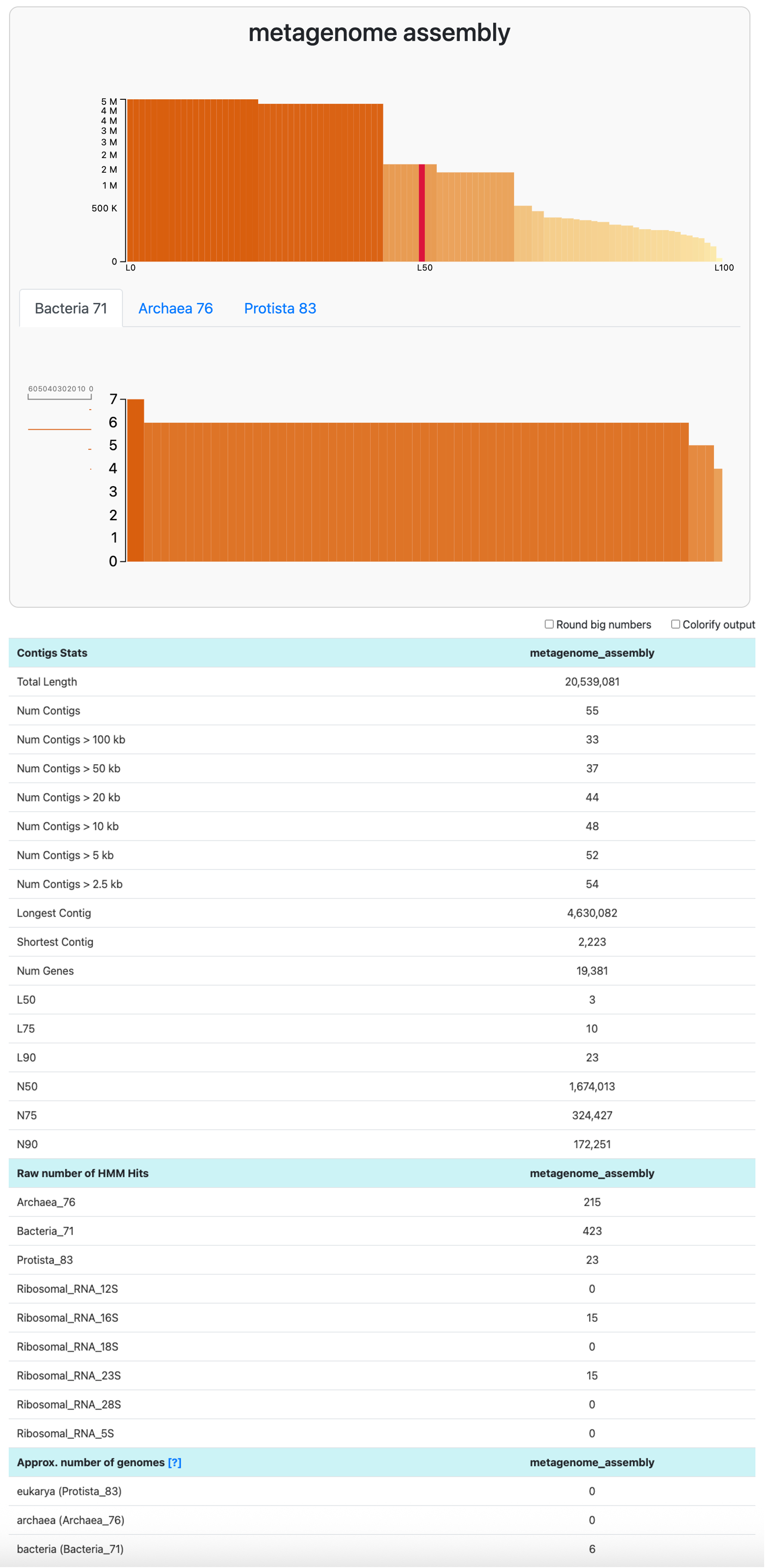
This assembly is estimated to contain six populations. To learn more about the composition of this metagenome, we can use anvi-estimate-scg-taxonomy with the flag --metagenome-mode. In this mode, anvi’o will not try to compute the consensus taxonomy of every ribosomal protein as it does by default. Instead, it will report the taxonomy of all the genes matching to the most abundant ribosomal protein:
$ anvi-estimate-scg-taxonomy -c 00_DATA/metagenome/sample01-contigs.db --metagenome-mode
Contigs DB ...................................: 00_DATA/sample01-contigs.db
Metagenome mode ..............................: True
SCG for metagenome ...........................: None

* A total of 132 single-copy core genes with taxonomic affiliations were
  successfully initialized from the contigs database 🎉 Following shows the
  frequency of these SCGs: Ribosomal_L1 (6), Ribosomal_L13 (6), Ribosomal_L14
  (6), Ribosomal_L16 (6), Ribosomal_L17 (6), Ribosomal_L19 (6), Ribosomal_L2
  (6), Ribosomal_L20 (6), Ribosomal_L21p (6), Ribosomal_L22 (6), Ribosomal_L27A
  (6), Ribosomal_L3 (6), Ribosomal_L4 (6), Ribosomal_L5 (6), Ribosomal_S11 (6),
  Ribosomal_S15 (6), Ribosomal_S16 (6), Ribosomal_S2 (6), Ribosomal_S6 (6),
  Ribosomal_S7 (6), Ribosomal_S8 (6), Ribosomal_S9 (6).

WARNING
===============================================
Anvi'o automatically set 'Ribosomal_L1' to be THE single-copy core gene to
survey your metagenome for its taxonomic composition. If you are not happy with
that, you could change it with the parameter `--scg-name-for-metagenome-mode`.


Taxa in metagenome "metagenome_assembly"
===============================================
+----------------------------------------+--------------------+--------------------------------------------------------------------------------------------------------------------------+
|                                        |   percent_identity | taxonomy                                                                                                                 |
+========================================+====================+==========================================================================================================================+
| metagenome_assembly_Ribosomal_L1_10579 |                100 | Bacteria / Pseudomonadota / Gammaproteobacteria / Pseudomonadales / Oleiphilaceae / Marinobacter / Marinobacter salarius |
+----------------------------------------+--------------------+--------------------------------------------------------------------------------------------------------------------------+
| metagenome_assembly_Ribosomal_L1_12451 |                100 | Bacteria / Cyanobacteriota / Cyanobacteriia / PCC-6307 / Cyanobiaceae / Prochlorococcus_A /                              |
+----------------------------------------+--------------------+--------------------------------------------------------------------------------------------------------------------------+
| metagenome_assembly_Ribosomal_L1_15984 |                100 | Bacteria / Pseudomonadota / Alphaproteobacteria / Rhizobiales / Stappiaceae / Roseibium / Roseibium aggregatum           |
+----------------------------------------+--------------------+--------------------------------------------------------------------------------------------------------------------------+
| metagenome_assembly_Ribosomal_L1_3513  |               99.6 | Bacteria / Pseudomonadota / Gammaproteobacteria / Enterobacterales_A / Alteromonadaceae / Alteromonas /                  |
+----------------------------------------+--------------------+--------------------------------------------------------------------------------------------------------------------------+
| metagenome_assembly_Ribosomal_L1_5126  |                100 | Bacteria / Pseudomonadota / Alphaproteobacteria / HIMB59 / HIMB59 / HIMB59 / HIMB59 sp000299115                          |
+----------------------------------------+--------------------+--------------------------------------------------------------------------------------------------------------------------+
| metagenome_assembly_Ribosomal_L1_5655  |               99.6 | Bacteria / Pseudomonadota / Alphaproteobacteria / Pelagibacterales / Pelagibacteraceae / Pelagibacter /                  |
+----------------------------------------+--------------------+--------------------------------------------------------------------------------------------------------------------------+
Alternatively, you can tell anvi’o you want to use another ribosomal protein. The output of the above comment is already telling us that each ribosomal protein is present six times, so any gene should do the job. You can also use the flag --report-scg-frequencies, which will write these frequencies into a text file.
A matrix output with multiple metagenomes
If you have multiple metagenomes, you can use the flag --matrix to get an output file that looks like this (example output at the genus level):
| taxon | sample01 | sample02 | sample03 | sample04 | sample05 | sample06 |
|---|---|---|---|---|---|---|
| Prochlorococcus | 1.00 | 1.00 | 1.00 | 1.00 | 1.00 | 1.00 |
| Synechococcus | 1.00 | 0 | 1.00 | 1.00 | 0 | 1.00 |
| Pelagibacter | 1.00 | 1.00 | 1.00 | 1.00 | 1.00 | 1.00 |
| SAR86 | 1.00 | 1.00 | 0 | 1.00 | 1.00 | 1.00 |
| SAR92 | 0 | 1.00 | 1.00 | 0 | 1.00 | 1.00 |
| SAR116 | 1.00 | 0 | 1.00 | 1.00 | 0 | 1.00 |
| Roseobacter | 0 | 1.00 | 1.00 | 0 | 1.00 | 0 |
Pangenomics
Show/Hide Starting the tutorial at this section? Click here for data preparation steps.
If you haven’t run previous sections of this tutorial (particularly the ‘Working with multiple genomes’ section), then you should follow these steps to setup the files that we will use going forward.
cp 00_DATA/contigs/*-contigs.db .
anvi-script-gen-genomes-file --input-dir . -o external-genomes.txt
Pangenomics represents a set of computational strategies to compare and study the relationship between a set of genomes through gene clusters. For a more comprehensive introduction into the subject, see this video.
Since the core concept of pangenomics is to compare genomes based on their gene content, it is important to know which genomes you plan you to use. Pangenomics is typically used with somewhat closely related organisms, at the species, genus, sometimes family level. It is also valuable to check the estimated completeness and overall quality of the genomes you want in include in your pangenome analysis.
Low completeness genomes are likely missing some portion of their gene content. For that reason, we will include 7 out of the 8 Trichodesmium genomes to compute a pangenome. We won’t use the Trichodesmium thiebautii H9_4 because of its low estimated completeness and overall smaller genome size.
The inputs will be the contigs databases that are present in the datapack, plus the contigs-db of the Trichodesmium MAG that you downloaded in the first part of this tutorial.
$ ls 00_DATA/contigs
MAG_Candidatus_Trichodesmium_miru-contigs.db     MAG_Trichodesmium_thiebautii_Atlantic-contigs.db Trichodesmium_sp-contigs.db
MAG_Candidatus_Trichodesmium_nobis-contigs.db    MAG_Trichodesmium_thiebautii_Indian-contigs.db   Trichodesmium_thiebautii_H9_4-contigs.db
MAG_Trichodesmium_erythraeum-contigs.db          Trichodesmium_erythraeum_IMS101-contigs.db
Genome storage
The first step to compute a pangenome in anvi’o is the command anvi-gen-genomes-storage, which takes multiple contigs databases as input and generates a new anvi’o database called the genomes-storage-db. This database holds all gene information like functional annotations and amino acid sequences in a single location.
The input to anvi-gen-genomes-storage is an external-genomes file. You should have one from the section about working with multiple genomes. We just need to remove the Trichodesmium thiebautii H9_4:
grep -v Trichodesmium_thiebautii_H9_4 external-genomes.txt > external-genomes-pangenomics.txt
Then we can use the command anvi-gen-genomes-storage:
# make a directory of the pangenome analysis
mkdir -p 01_PANGENOME
anvi-gen-genomes-storage -e external-genomes-pangenomics.txt -o 01_PANGENOME/Trichodesmium-GENOMES.db
Pangenome analysis
To actually run the pangenomic analysis, we will use the command anvi-pan-genome. The sole input is the genomes-storage-db and it will generate a new database, called the pan-db:
# will a few min
anvi-pan-genome -g 01_PANGENOME/Trichodesmium-GENOMES.db \
                -o 01_PANGENOME \
                -n Trichodesmium \
                -T 4
Under the hood, anvi-pan-genome uses DIAMOND (or BLASTp if you choose the alternative) to compute the similarity between amino acid sequences from every genomes. From this all-vs-all search, it will use the MCL algorithm to cluster the genes into groups of relatively high similarity. The pan-db stores the gene cluster information.
Interactive pangenomics display
Now that we have a genomes-storage-db and a pan-db, we can use the command anvi-display-pan to start an interactive interface of our pangenome:
anvi-display-pan -g 01_PANGENOME/Trichodesmium-GENOMES.db -p 01_PANGENOME/Trichodesmium-PAN.db
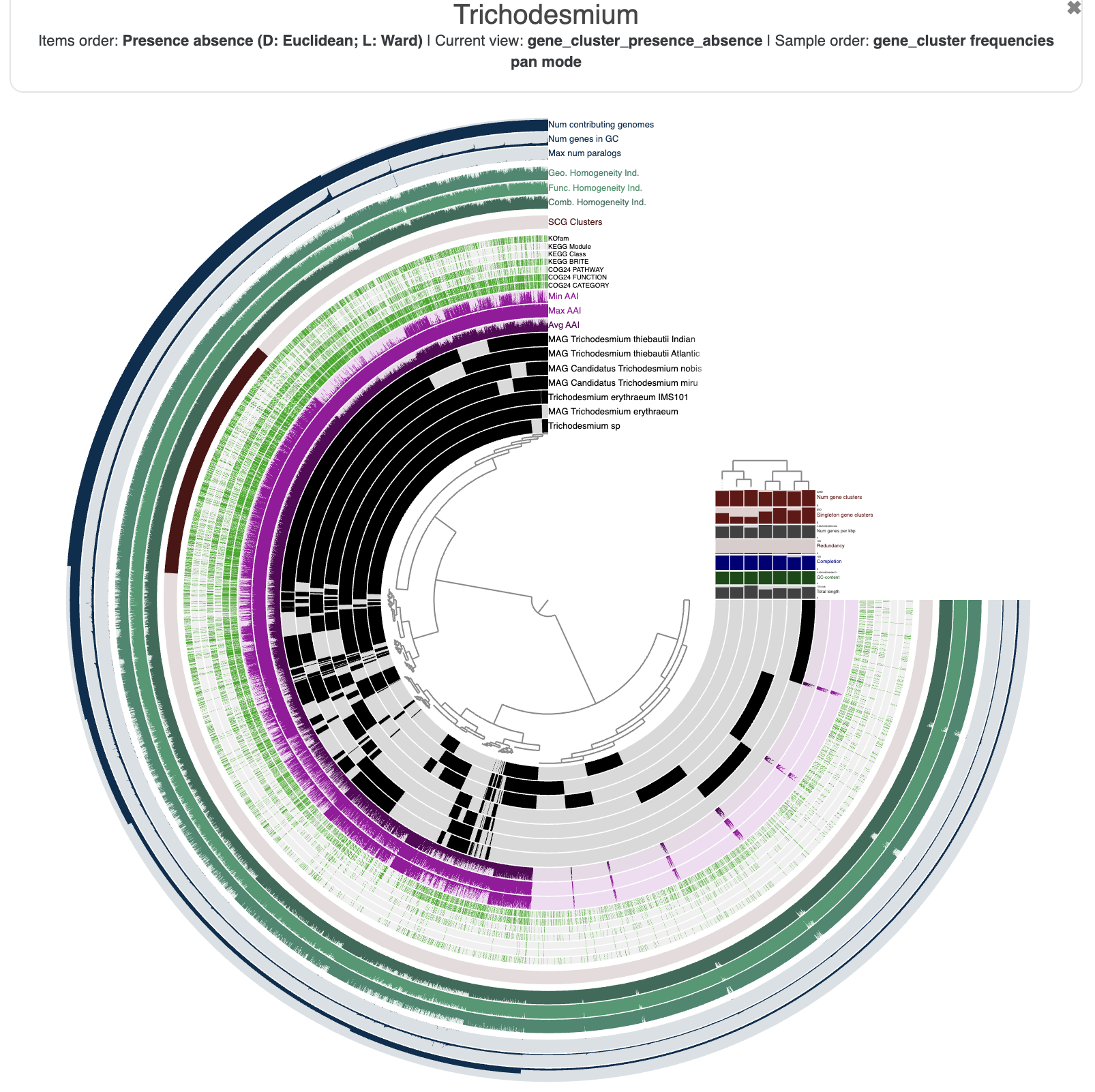
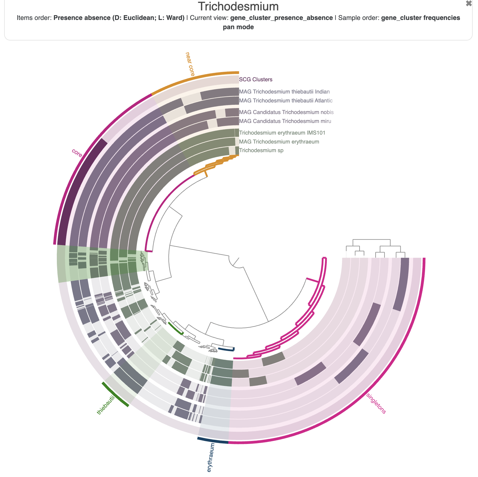
And here is what you should see in your browser:
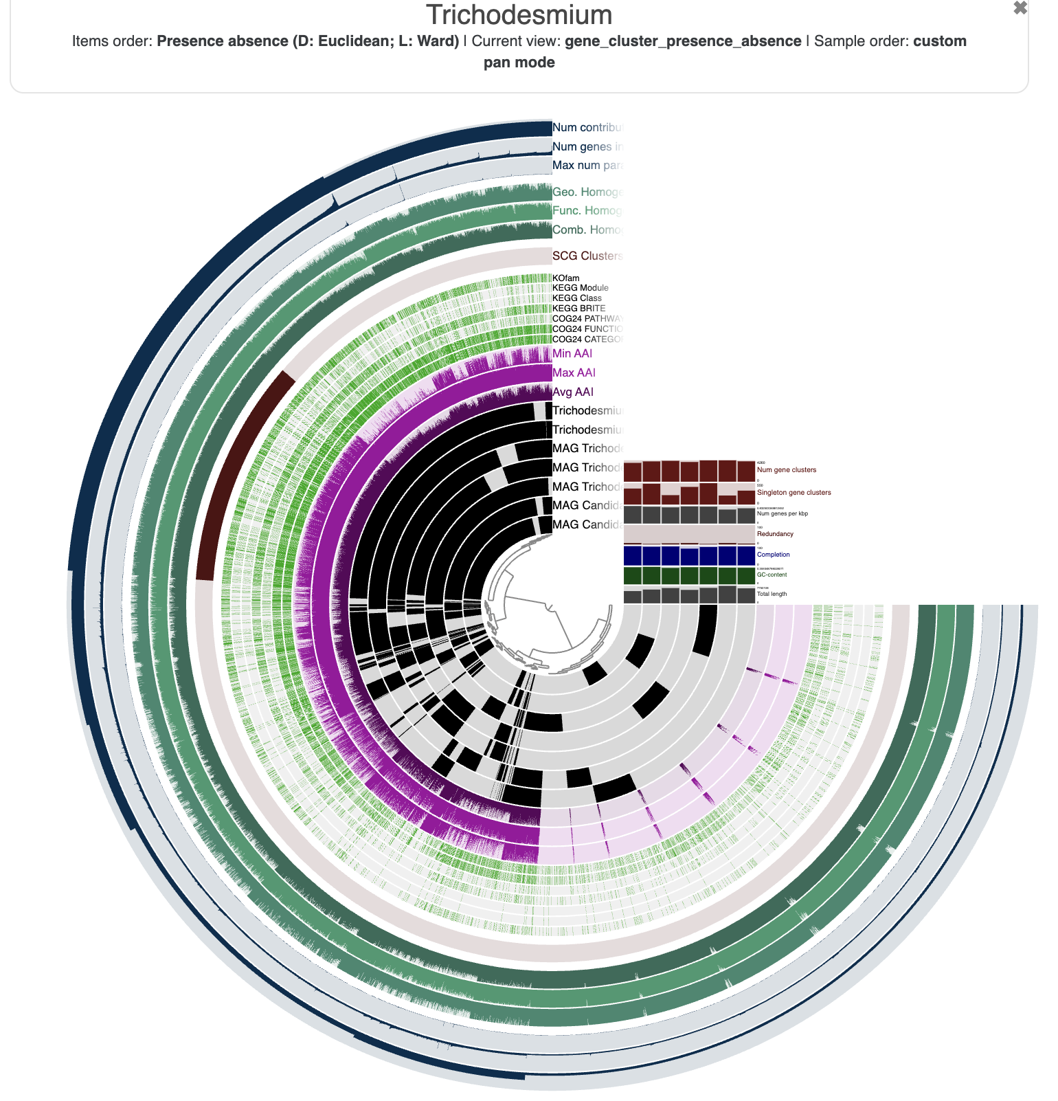
You are seeing:
- The genomes in black layers.
- The inner dendrogram: every leaf of that dendrogram is a gene cluster.
- The black heatmap: presence/absence of a gene from a genome in a gene cluster.
- Multiple colorful additional layers with information about the underlying gene cluster.
- Some layer (genome) data at the right-end of the circular heatmap.
First of all, let’s reorder the genomes. By default they will simply appear in alphabetical order, which is not very interesting. In the main panel, you can scroll down to “Layers” and select gene_cluster_frequency:
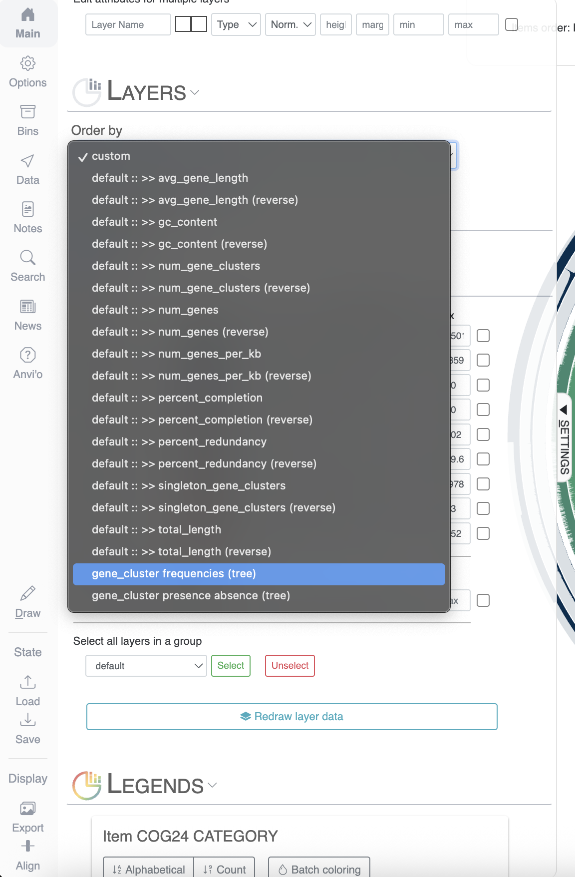
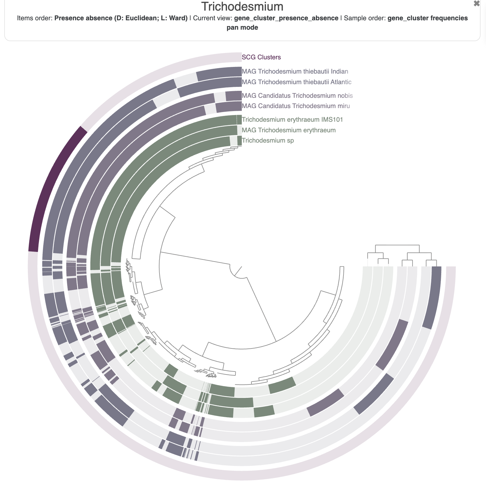
The resulting figure will now pull together genomes that share similar gene content. It may not be very noticeable at first but if you pay attention between the before/after you will notice that we have now two clusters (see dendrogram on the right):
This figure was made with a dendrogram radius of 4500. You can change the radius in the Options tab.
Now that you have made some modifications to your interactive figure, it would be a good idea to save those settings. The aesthetics of a figure are saved in a “State”, and you will find a button on the bottom left of the interface to save it. You can store multiple states for the same pangenome (different colors, different layers being displayed, etc). The state called default will always be the one displayed when you start an interactive interface. The state can also be exported/imported from the terminal with the programs anvi-export-state and anvi-import-state.
You can spend some time getting familiar with the interface and all the possible customisation options. For instance, here is the pangenome figure I made:
The state to reproduce the figure above is available in the directory 00_DATA, and you can import it with the following command:
anvi-import-state -p 01_PANGENOME/Trichodesmium-PAN.db -s 00_DATA/pan_state.json -n tutorial_state
Inspect gene clusters
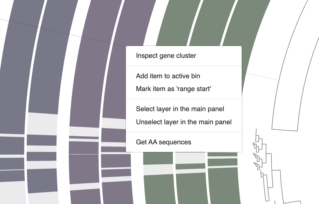
Every gene cluster contains one or more amino acid sequences from one or more genomes. In some cases, they may contain multiple genes from a single genome (i.e., multi-copy genes). You can use your mouse and select a gene cluster on the interface, right-click and select Inspect gene cluster:
It will open a new tab with the multisequence alignment of the amino acid sequences in the cluster:
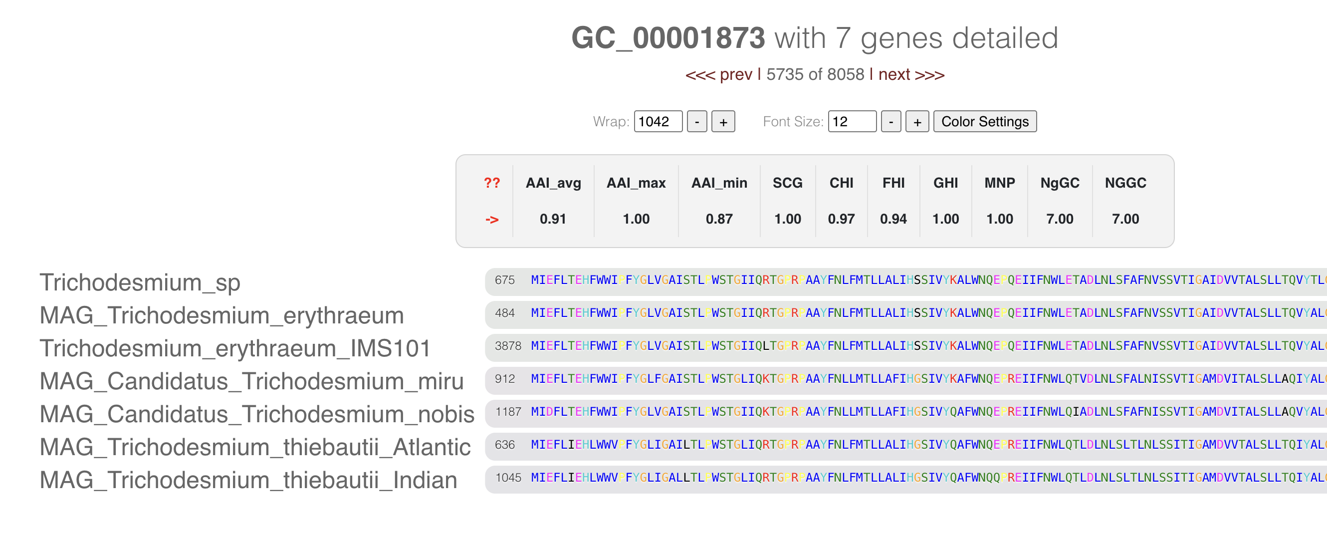
If you want to know more about the amino acid coloring, you can check this blog post by Mahmoud Yousef. In brief, the colors represent the amino acid properties (like polar, cyclic) and their conservancy in the alignment.
If you click on one of the gene caller ID numbers you will get some information about that gene:
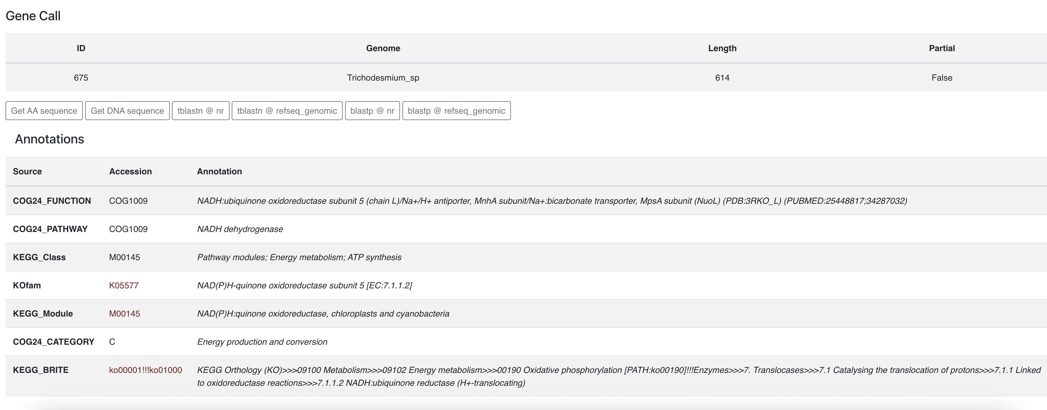
From there you can learn about its functional annotations, if any. You can also retrieve the amino acid sequence and start some BLAST commands on the NCBI servers.
Bin and summarize a pangenome
Looking at individual genes clusters is great, but not very practical to summarize a large selection of gene clusters. Fortunately for you, you can select gene clusters in the main interface and create ‘bins’ which you can meaningfully rename. In the next screenshot, I have selected the core genome, the near core, the accessory genome of Trichodesmium erythraeum * and *Trichodesmium thiebautii, and all the singleton gene clusters.
Once you are happy with your bins, don’t forget to save them into a collection. Just like the ‘state’ saves the current settings for the figure, the ‘collection’ stores your selection of items, here gene clusters. You can save as many collections as you want, and the collection called default will always appear when you start the interactive interface with anvi-display-pan.
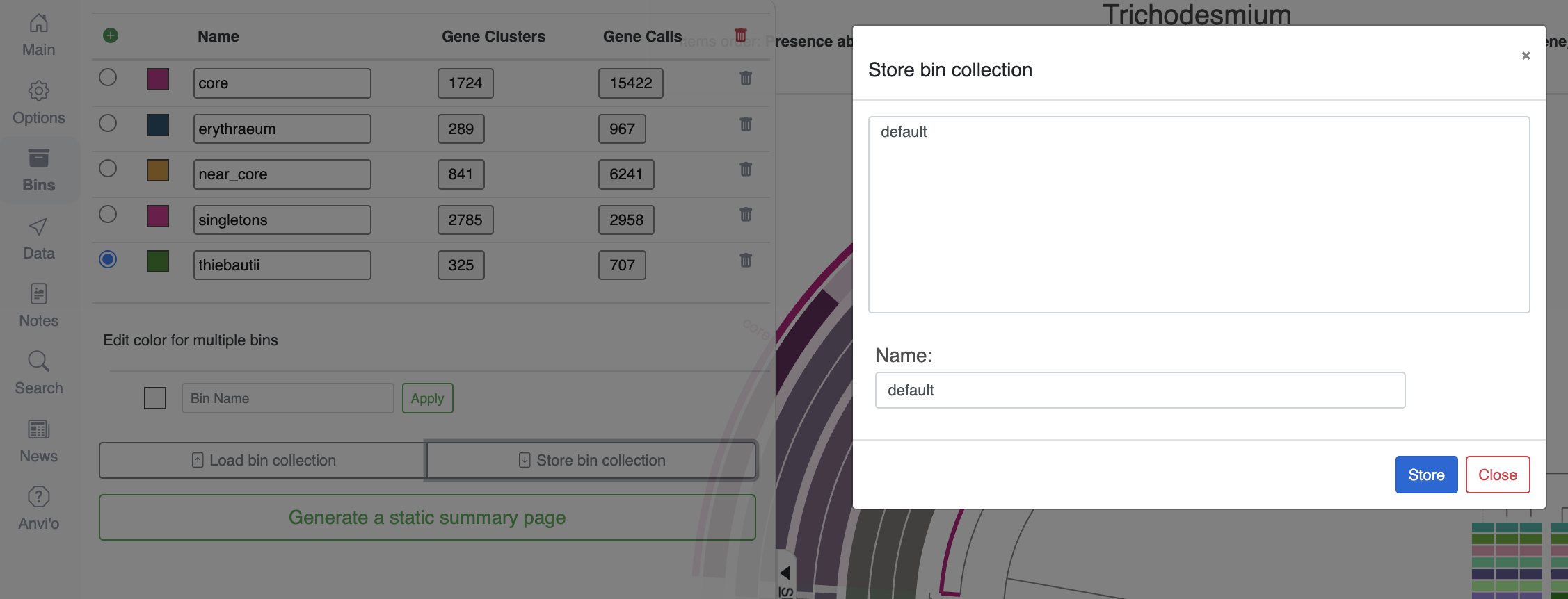
Now that we have some meaningful bins, it is time to make sense of their content by either using the program anvi-summarize, or selecting Generate a static summary page in the “Bins” tab of the interface.
Here is how you would do it with the command line (note that I named my collection “default”):
anvi-summarize -g 01_PANGENOME/Trichodesmium-GENOMES.db \
               -p 01_PANGENOME/Trichodesmium-PAN.db \
               -C default \
               -o 01_PANGENOME/SUMMARY
The interactive interface button and the above command generate the same output directory, which contains a large table summarizing ALL genes from all genomes. Here are the first few rows:
unique_id |
gene_cluster_id |
bin_name |
genome_name |
gene_callers_id |
num_genomes_gene_cluster_has_hits |
num_genes_in_gene_cluster |
max_num_paralogs |
SCG |
functional_homogeneity_index |
geometric_homogeneity_index |
combined_homogeneity_index |
AAI_min |
AAI_max |
AAI_avg |
COG24_PATHWAY_ACC |
COG24_PATHWAY |
COG24_FUNCTION_ACC |
COG24_FUNCTION |
KEGG_BRITE_ACC |
KEGG_BRITE |
KOfam_ACC |
KOfam |
COG24_CATEGORY_ACC |
COG24_CATEGORY |
KEGG_Class_ACC |
KEGG_Class |
KEGG_Module_ACC |
KEGG_Module |
aa_sequence |
|---|---|---|---|---|---|---|---|---|---|---|---|---|---|---|---|---|---|---|---|---|---|---|---|---|---|---|---|---|---|
| 1 | GC_00000001 | near_core | MAG_Candidatus_Trichodesmium_miru | 3624 | 6 | 221 | 214 | 0 | 0.659555877418382 | 0.940765773081969 | 0.775453602988201 | 0.12124248496994 | 1.0 | 0.956257104913241 | ——————————————————————————————————————————————————————————————————————————————————————————————————————————————————————————————————————————————————MQSWAAEELKYTNLPDKRLNQRLIKIVEQASAQPEASVPQASGDWANTKATYYFWNSERFSSEDIIDGHRRSTAQRASQEDVILAIQDTSDFNFTHHKGKTWDKGFGQTCSQKYVRGLKVHSTLAVSSQGVPLGILDLQIWTREPNKKRKKKKSKGSTSIFNKESKRWLRGLVDAELAIPSTTKIVTIADREGDMYELFALVILANSELLIRANHNRRVNHEMKYLRDRFSQAPEAGKLKVSVPKKDGQPLREATLSIRYGMLTICAPNNLSQGNNRSPITLNVISAVEENFAEGVKPINWLLLTTKEVDNFEDAVGCIRWYTYRWLIERYHYVLKSGCGIEKLQLKTAQRIKKALATYALVAWRLLWLTYHGRENPQLKSDKVLEQHEWQSLYCHFHCTSIAPAQPPSLKQAMVWIAKLGGFLGRKNDGEPGVKSLWRGLKRLHDIASTWKLAHSSTSIACESYR———————————————————————————————- | ||||||||||||||
| 2 | GC_00000001 | near_core | MAG_Candidatus_Trichodesmium_nobis | 940 | 6 | 221 | 214 | 0 | 0.659555877418382 | 0.940765773081969 | 0.775453602988201 | 0.12124248496994 | 1.0 | 0.956257104913241 | ——————————————————————————————————————————————————————————————————————————————————————————————————————————————————————————————————————————————————MQSWAAEELKYTNLPDKRLNQRLIKIVEQASAQPEASVPQASGDWANTKATYYFWNSERFSSEDIIDGHRRSTAQRASQEDVILAIQDTSDFNFTHHKGKTWDKGFGQTCSQKYVRGLKVHSTLAVSSQGVPLGILDLQIWTREPNKKRKKKKSKGSTSIFNKESKRWLRGLVDAELAIPSTTKIVTIADREGDMYELFALVILANSELLIRANHNRRVNHEMKYLRESISQAPEAGKLKVSVPKKDGQPLREATLSIRYGMLTISASNNLSQGNNRSPITLNVIYAVEENFAEGVKPINWLLLTTKEVDNFEDAVGCIRWYTYRWLIERYHYVLKSGCGIEKLQLETAQRIKKALATYALVAWRLLWLTYHGRENPQLKSDTVLEQHEWQSLYCHFHCTSIAPAQPPSLKQAMVWIAKLGGFLGRKNDGEPGVKSLWRGLKRLHDIASTWKLAHSSTSIACESYG———————————————————————————————- | ||||||||||||||
| 3 | GC_00000001 | near_core | MAG_Candidatus_Trichodesmium_nobis | 682 | 6 | 221 | 214 | 0 | 0.659555877418382 | 0.940765773081969 | 0.775453602988201 | 0.12124248496994 | 1.0 | 0.956257104913241 | ———————————————————————————————————————————————————————————————————————————————————————————————————————————————————————————————————————————MVWIAKLGGFLGSKNDGEPGVKSLW————————————————————————————————————————————————————————————————————————————————————————————————————————————————————————————————————————————————–RVLERLYDIASTWKLIHSSTSIACESYG———————————————————————————————- | ||||||||||||||
| 4 | GC_00000001 | near_core | MAG_Trichodesmium_erythraeum | 90 | 6 | 221 | 214 | 0 | 0.659555877418382 | 0.940765773081969 | 0.775453602988201 | 0.12124248496994 | 1.0 | 0.956257104913241 | ——————————————————————————————————————————————————————————————————————————————————————————————————————————————————————————————————————————–AMVWIAKLGGFLGRKNDGEPGVKSLW————————————————————————————————————————————————————————————————————————————————————————————————————————————————————————————————————————————————–RGLKRLHDIASTWKLAHSFTSIACESYG———————————————————————————————- | ||||||||||||||
| 5 | GC_00000001 | near_core | MAG_Trichodesmium_erythraeum | 143 | 6 | 221 | 214 | 0 | 0.659555877418382 | 0.940765773081969 | 0.775453602988201 | 0.12124248496994 | 1.0 | 0.956257104913241 | ——————————————————————————————————————————————————————————————————————————————————————————————————————————————————————————————————————————–AMVWIAKLGGFLGRKNDGEPGVKSLW————————————————————————————————————————————————————————————————————————————————————————————————————————————————————————————————————————————————–RGLKRLHDIASTWKLAHSFTSIACESYG———————————————————————————————- | ||||||||||||||
| 6 | GC_00000001 | near_core | MAG_Trichodesmium_erythraeum | 334 | 6 | 221 | 214 | 0 | 0.659555877418382 | 0.940765773081969 | 0.775453602988201 | 0.12124248496994 | 1.0 | 0.956257104913241 | ——————————————————————————————————————————————————————————————————————————————————————————————————————————————————————————————————————————–AMVWIAKLGGFLGRKNDGEPGVKSLW————————————————————————————————————————————————————————————————————————————————————————————————————————————————————————————————————————————————–RGLKRLHDIASTWKLAHSFTSIACESYG———————————————————————————————- | ||||||||||||||
| 7 | GC_00000001 | near_core | MAG_Trichodesmium_erythraeum | 601 | 6 | 221 | 214 | 0 | 0.659555877418382 | 0.940765773081969 | 0.775453602988201 | 0.12124248496994 | 1.0 | 0.956257104913241 | ——————————————————————————————————————————————————————————————————————————————————————————————————————————————————————————————————————————–AMVWIAKLGGFLGRKNDGEPGVKSLW————————————————————————————————————————————————————————————————————————————————————————————————————————————————————————————————————————————————–RGLKRLHDIASTWKLAHSFTSIACESYG———————————————————————————————- | ||||||||||||||
| 8 | GC_00000001 | near_core | MAG_Trichodesmium_erythraeum | 901 | 6 | 221 | 214 | 0 | 0.659555877418382 | 0.940765773081969 | 0.775453602988201 | 0.12124248496994 | 1.0 | 0.956257104913241 | ——————————————————————————————————————————————————————————————————————————————————————————————————————————————————————————————————————————–AMVWIAKLGGFLGRKNDGEPGVKSLW————————————————————————————————————————————————————————————————————————————————————————————————————————————————————————————————————————————————–RGLKRLHDIASTWKLAHSFTSIACESYG———————————————————————————————- | ||||||||||||||
| 9 | GC_00000001 | near_core | MAG_Trichodesmium_erythraeum | 917 | 6 | 221 | 214 | 0 | 0.659555877418382 | 0.940765773081969 | 0.775453602988201 | 0.12124248496994 | 1.0 | 0.956257104913241 | ——————————————————————————————————————————————————————————————————————————————————————————————————————————————————————————————————————————–AMVWIAKLGGFLGRKNDGEPGVKSLW————————————————————————————————————————————————————————————————————————————————————————————————————————————————————————————————————————————————–RGLKRLHDIASTWKLAHSFTSIACESYG———————————————————————————————- |
Search for functional annotations
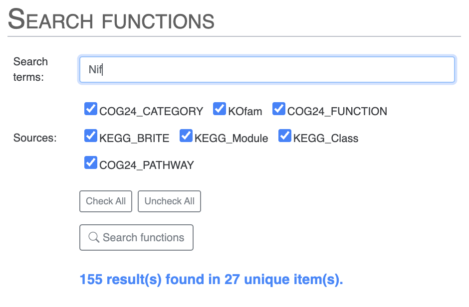
If you are interested in one or more functional annotations and where they fit in the pangenome - core, accessory, singleton, single or multiple copies - then you can use the “Search” tab. There you can search using any term you like. You can search for Nif and you will get all Nif genes, including NifH and more.
Or, you can directly search for NifH and you will notice two results which are not expected. We know from Tom’s paper that COG miss-annotates a ferredoxin gene as NifH:
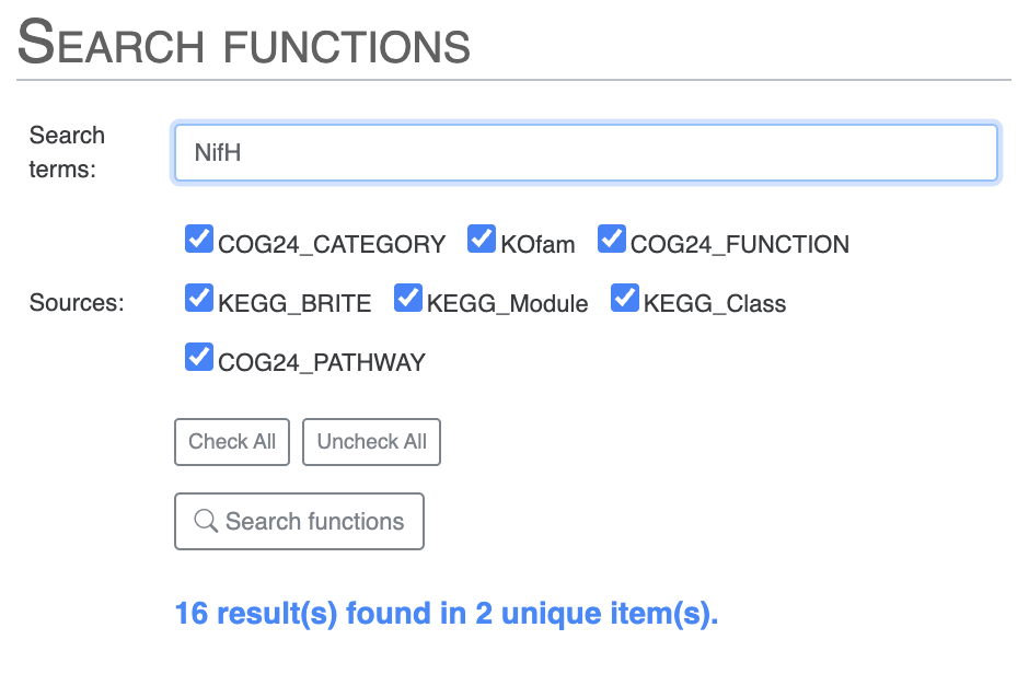
For instance, we found that genes with COG20 function incorrectly annotated as “Nitrogenase ATPase subunit NifH/coenzyme F430 biosynthesis subunit CfbC” correspond, in reality, to “ferredoxin: protochlorophyllide reductase.”
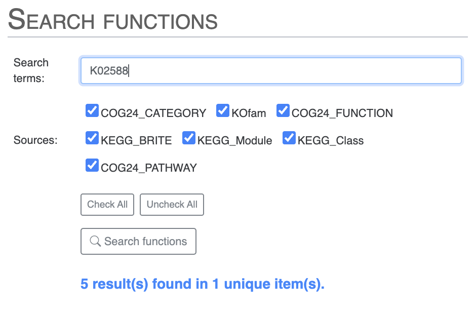
Then you can search for NifH by selecting only the KOfam annotation source, or directly use the KOfam accession number K02588:
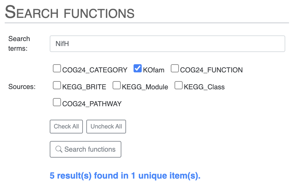
Then you can scroll down to where you can list the results of the search or choose to highlight them on the pangenome. I would suggest you look for all the Nif genes, using only the KOfam annotation source to avoid the issues with COG. Then highlight the results on your pangenome. You can even choose to add the search result items to a bin.
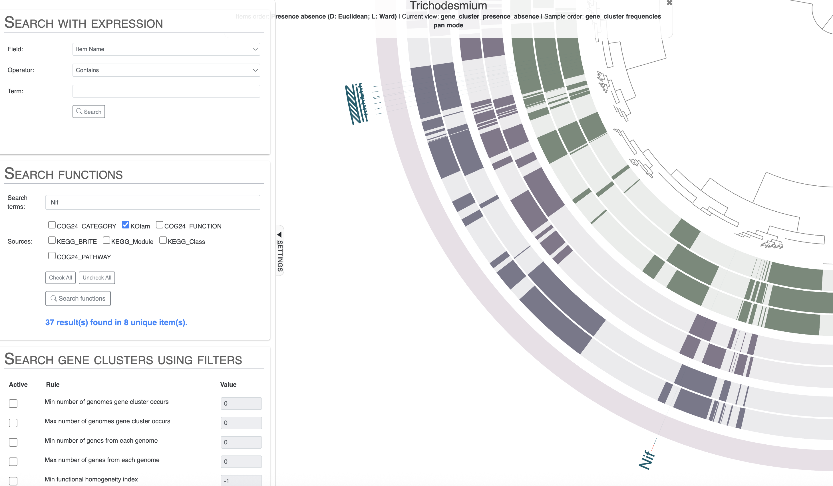
Note how nearly all Nif genes are concentrated in a section of the pangenome which correspond to gene clusters shared between Trichodesmium thiebautii and erythraeum, and not in Trichodesmium miru or nobis. The result is coherent with these genomes lacking nitrogen fixation capabilities, but you may be wondering what is happening for that single gene cluster on the lower part of the pangenome. It is found in T. miru, T. nobis and one T. thiebautii. If you inspect that gene cluster and look for the full functional annotation, you will see that it is NifU, which is not a marker for nitrogen fixation as it can be found in non-diazotrophic organisms.
Additional genome information
To help make sense of your pangenome, you can add multiple additional data layers with information about the genomes you are using. We will see how you can add the taxonomy information that we computed earlier, and also the pairwise average nucleotide identity of these genomes.
Add taxonomy
We previously used anvi-estimate-scg-taxonomy and made a text output called taxonomy_multi_genomes.txt. We can import that table directly into the pangenome with the command anvi-import-misc-data:
anvi-import-misc-data -p 01_PANGENOME/Trichodesmium-PAN.db \
                      -t layers \
                      --just-do-it \
                      taxonomy_multi_genomes.txt
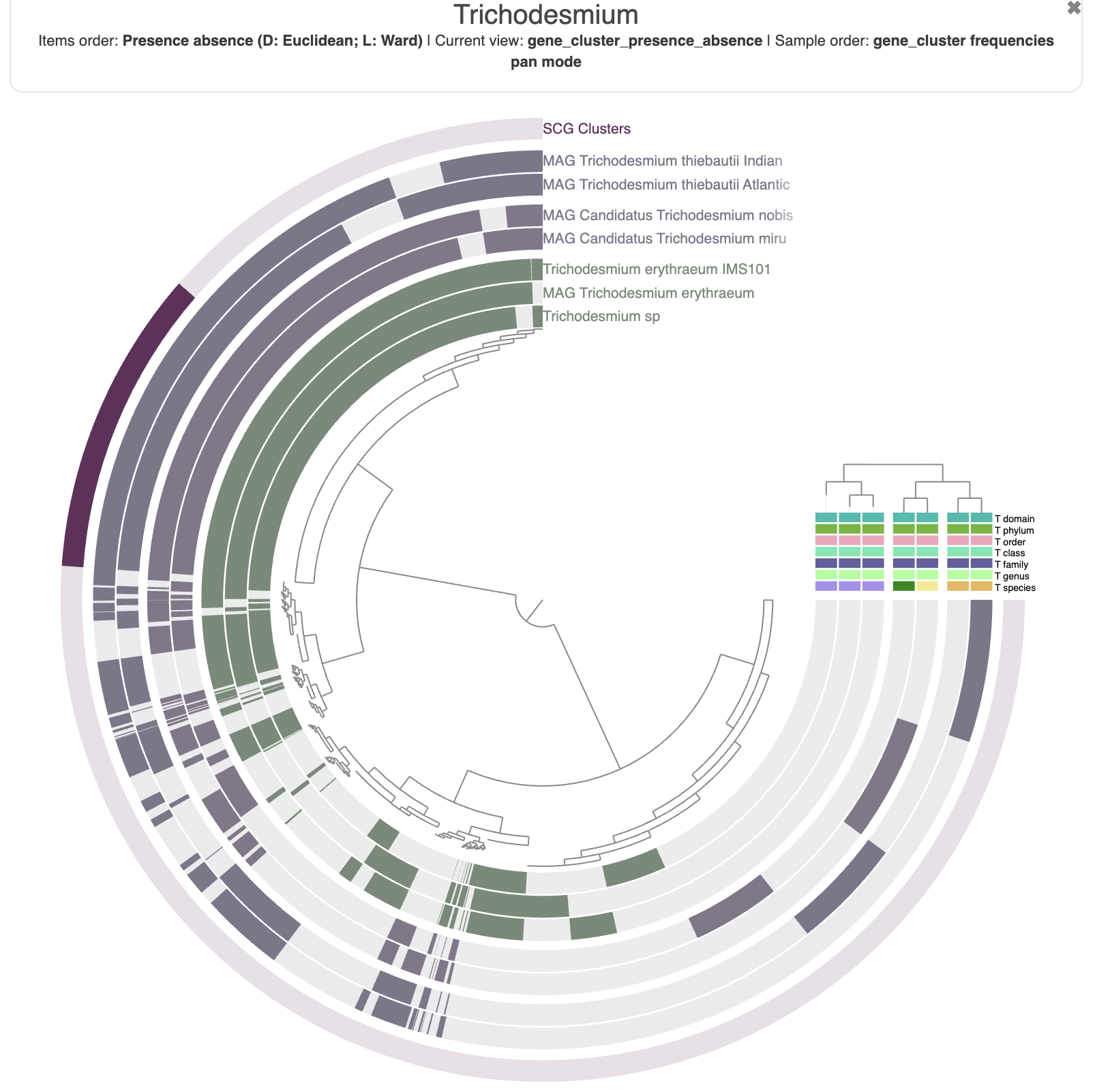
Nothing very surprising, but it is always good to see that the taxonomy agrees with how the genomes are currently organized, i.e. by their gene content.
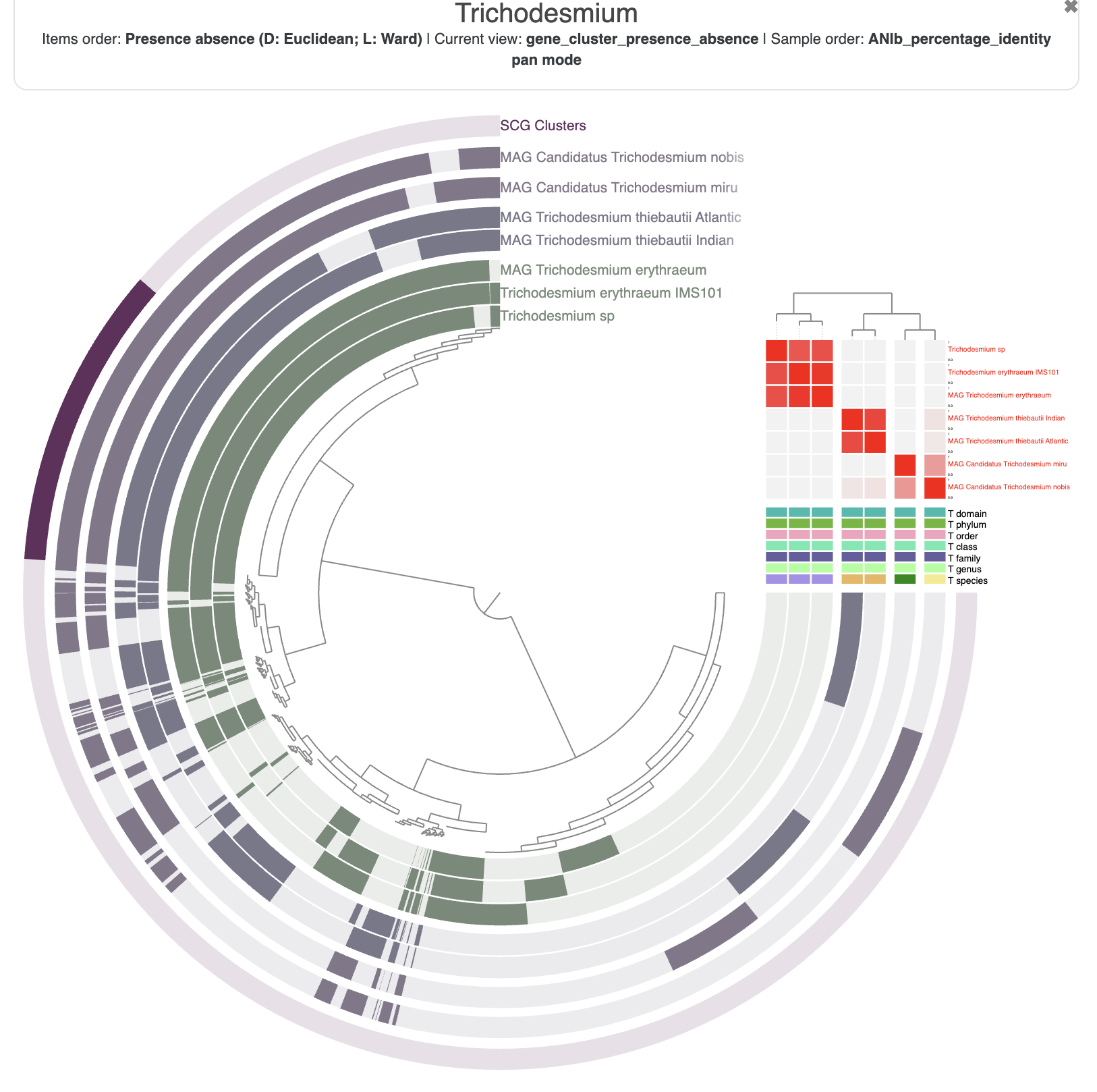
Compute average nucleotide identity
A companion metric to pangenomes is the Average Nucleotide Identity, or ANI, which is based on whole genome DNA similarity. There is a program called anvi-compute-genome-similarity that allows you to use your contigs-db and three different methods to compute ANI. By default it uses PyANI, but you can also choose FastANI.
The sole required input is an external-genomes file, and the output is a directory with multiple files containing the ANI value, coverage, and more. Optionally, you can also provide a pan-db and anvi’o will import the ANI values directly into your pangenome.
anvi-compute-genome-similarity -e external-genomes-pangenomics.txt \
                               -p 01_PANGENOME/Trichodesmium-PAN.db \
                               -o 01_PANGENOME/ANI \
                               --program pyANI \
                               -T 4
You should check the content of the output directory, 01_PANGENOME/ANI. It contains multiple matrices and associated tree files.
A friendly reminder that the ANI is computed on the fraction of two genomes that align to each other. Any genomic segment that is not found in one of the genomes is not taken into account in the final percent identity. The output of PyANI includes the alignment coverage of the pairwise genome comparison, and also the full_percentage_identity which correspond to ANI * coverage. Also note that ANI is not a symmetrical value.
When you start the interactive interface with anvi-display-pan, you should be able to select the ANI identity values in the layer section of the main panel. You can also reorder the genomes based on the ANI similarities in the “layers” section of the main table.
Integrating ecology and evolution with metapangenome
AS you can see from the example above, you can integrate a lot of information in a single anvi’o figure. And not just the figure, as the pan-db contains all the information in the interactive display as well.
Another topic not covered yet in this tutorial is metagenomic read recruitment, which allows you to compute detection and coverage of one or more genomes across metagenomes. This gives you an ecological signal and nothing is stopping you from importing a relative abundance heatmap, just like the ANI. There is a dedicated function in anvi’o, called anvi-meta-pan-genome, which you can learn more about here.
At the end of the day, you can have a figure like this one, with ecology and evolution integrated in one figure:
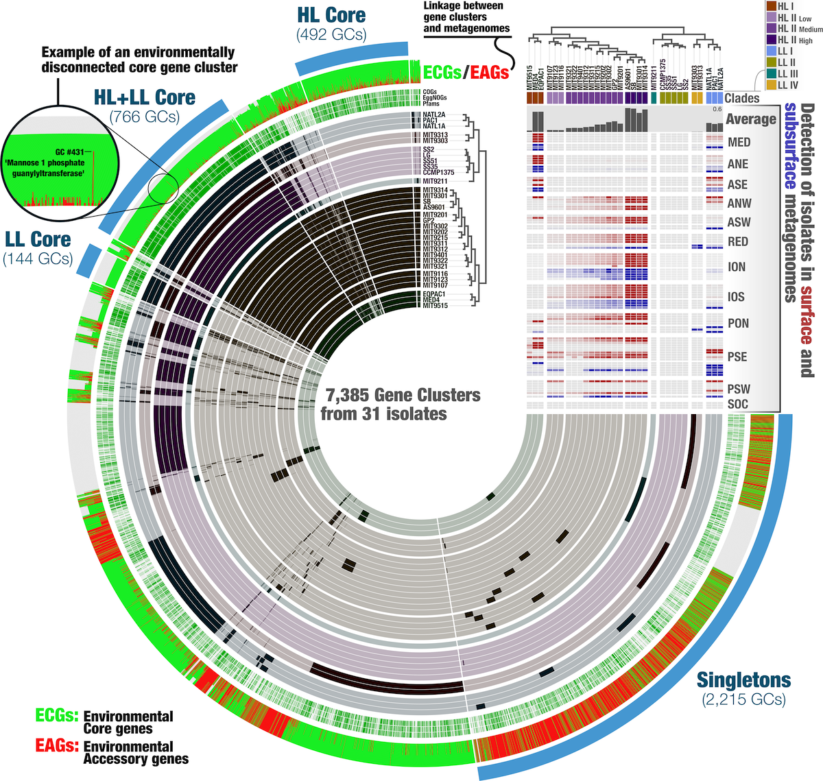
But that analysis is for another time.
Metabolism
Show/Hide Starting the tutorial at this section? Click here for data preparation steps.
If you haven’t run previous sections of this tutorial (particularly the ‘Working with multiple genomes’ section), then you should follow these steps to setup the files that we will use going forward.
cp 00_DATA/contigs/*-contigs.db .
anvi-script-gen-genomes-file --input-dir . -o external-genomes.txt
ls 00_DATA/fasta | cut -d "." -f1 > genomes.txt
Looking at individual gene functions is undisputably useful for understanding the lifestyle and potential activities of microbes. However, most genes do not work in isolation. Metabolic capacities such as nitrogen fixation, photosynthesis, biosynthesis of cellular components, and carbon utilization require multiple enzymes (or enzyme components) working sequentially or in parallel to catalyze all chemical reactions in a so-called metabolic pathway. In many cases, there are also several possible versions of these enzymes – variants across different domains of life, taxonomic groups, or environmental conditions – that could be used to catalyze the same set of chemical reactions. Manually looking for all possible versions of all enzymes needed for a given metabolic capacity is possible (we just did it in the pangenomics section for nitrogen fixation), but it isn’t very efficient (and requires you to know exactly what you are looking for). And that sort of approach is unscaleable when you are interested in more than a handful of specific metabolic pathways.
This section of the tutorial covers metabolism reconstruction, a strategy for summarizing all the metabolic capacities of a given organism (or community) by examining functional annotations in their metabolic context. To do this, one can either aggregate the genes related to multiple individual metabolic pathways to evaluate the organism’s capacity to do specific, ecologically-relevant things (“pathway prediction”) or use all annotated enzymes to create the entire network of chemical reactions that the organism can catalyze (“metabolic modeling”).
To keep things organized, we’ll make a new subdirectory for ourselves in which we can work. We’ll copy the external genomes file in here for convenience.
mkdir -p 02_METABOLISM && cd 02_METABOLISM/
cp ../external-genomes.txt .
Estimating metabolic pathway completeness
We’ll start with pathway prediction. The program anvi-estimate-metabolism computes completeness scores (and copy numbers) of metabolic modules. By default, it uses modules from the KEGG MODULE database, which contains a lot of well-studied metabolic pathways of general interest that are defined in terms of KEGG Ortholog (KO) protein families. When you run anvi-setup-kegg-data to get the KEGG KOfam models used for annotation with anvi-run-kegg-kofams, you also set up the KEGG MODULE data on your computer.
Show/Hide What version of KEGG data do you have?
The KEGG database goes through regular updates, so to keep things a bit more stable anvi’o uses prepackaged snapshots of KEGG data. More reasons for this are explained here. You can have multiple different snapshots on your computer at the same time, and pick which one to use with the --kegg-data-dir parameter of KEGG-associated programs.
To keep track of which KEGG snapshot is relevant to your current dataset, anvi’o hashes the contents of the KEGG data directory and stores this hash in your contigs-db when you run anvi-run-kegg-kofams. You can see which version you have by running anvi-db-info and looking for the modules_db_hash key. For example, all of the Trichodesmium genomes in the tutorial datapack should have the following hash value:
modules_db_hash ..............................: 66e53d49e65a
This hash enables us to ensure that the version of KEGG used to annotate your (meta)genome matches to the version used for metabolism reconstruction.
The modules-db in the KEGG snapshot with hash 66e53d49e65a is strangely very slow to access from anvi’o programs that use it (like anvi-estimate-metabolism). We are still trying to figure out what is going on. In the meantime, program execution time is much longer than usual when using this version of KEGG :(
anvi-estimate-metabolism can work on individual genomes, but we’re interested in comparing the metabolic capacity of all 8 Trichodesmium genomes. So let’s use our handy-dandy external-genomes file to individually estimate metabolism on each one:
# takes 12 minutes
anvi-estimate-metabolism -e external-genomes.txt -O tricho_metabolism
You should get an output file called tricho_metabolism_modules.txt that looks like this:
module |
genome_name |
db_name |
module_name |
module_class |
module_category |
module_subcategory |
module_definition |
stepwise_module_completeness |
stepwise_module_is_complete |
pathwise_module_completeness |
pathwise_module_is_complete |
proportion_unique_enzymes_present |
enzymes_unique_to_module |
unique_enzymes_hit_counts |
enzyme_hits_in_module |
gene_caller_ids_in_module |
warnings |
|---|---|---|---|---|---|---|---|---|---|---|---|---|---|---|---|---|---|
| M00001 | MAG_Candidatus_Trichodesmium_miru | MAG_Candidatus_Trichodesmium_miru | Glycolysis (Embden-Meyerhof pathway), glucose => pyruvate | Pathway modules | Carbohydrate metabolism | Central carbohydrate metabolism | “(K00844,K12407,K00845,K25026,K00886,K08074,K00918) (K01810,K06859,K13810,K15916) (K00850,K16370,K21071,K24182,K00918) (K01623,K01624,K11645,K16305,K16306) K01803 ((K00134,K00150) K00927,K11389) (K01834,K15633,K15634,K15635) (K01689,K27394) (K00873,K12406)” | 1.0 | True | 1.0 | True | NA | No enzymes unique to module | NA | K00134,K00134,K00845,K00845,K00873,K00927,K01623,K01624,K01689,K01803,K01803,K01810,K01834,K15633,K21071,K25026 | 2899,2579,3691,4200,985,2838,2319,1760,2136,3621,4011,2573,2274,2197,1300,1049 | K00134 is present in multiple modules: M00001/M00002/M00003/M00308/M00552/M00165/M00611/M00612,K00845 is present in multiple modules: M00001/M00549,K00873 is present in multiple modules: M00001/M00002,K00927 is present in multiple modules: M00001/M00002/M00003/M00308/M00552/M00165/M00611/M00612,K01623 is present in multiple modules: M00001/M00003/M00165/M00611/M00612,K01624 is present in multiple modules: M00001/M00003/M00165/M00345/M00344/M00611/M00612,K01689 is present in multiple modules: M00001/M00002/M00003/M00346,K01803 is present in multiple modules: M00001/M00002/M00003/M00165,K01810 is present in multiple modules: M00001/M00004,K01834 is present in multiple modules: M00001/M00002/M00003,K15633 is present in multiple modules: M00001/M00002/M00003,K21071 is present in multiple modules: M00001/M00345,K25026 is present in multiple modules: M00001/M00549 |
| M00002 | MAG_Candidatus_Trichodesmium_miru | MAG_Candidatus_Trichodesmium_miru | Glycolysis, core module involving three-carbon compounds | Pathway modules | Carbohydrate metabolism | Central carbohydrate metabolism | “K01803 ((K00134,K00150) K00927,K11389) (K01834,K15633,K15634,K15635) (K01689,K27394) (K00873,K12406)” | 1.0 | True | 1.0 | True | NA | No enzymes unique to module | NA | K00134,K00134,K00873,K00927,K01689,K01803,K01803,K01834,K15633 | 2899,2579,985,2838,2136,3621,4011,2274,2197 | K00134 is present in multiple modules: M00001/M00002/M00003/M00308/M00552/M00165/M00611/M00612,K00873 is present in multiple modules: M00001/M00002,K00927 is present in multiple modules: M00001/M00002/M00003/M00308/M00552/M00165/M00611/M00612,K01689 is present in multiple modules: M00001/M00002/M00003/M00346,K01803 is present in multiple modules: M00001/M00002/M00003/M00165,K01834 is present in multiple modules: M00001/M00002/M00003,K15633 is present in multiple modules: M00001/M00002/M00003 |
| M00003 | MAG_Candidatus_Trichodesmium_miru | MAG_Candidatus_Trichodesmium_miru | Gluconeogenesis, oxaloacetate => fructose-6P | Pathway modules | Carbohydrate metabolism | Central carbohydrate metabolism | “(K01596,K01610) (K01689,K27394) (K01834,K15633,K15634,K15635) K00927 (K00134,K00150) K01803 ((K01623,K01624,K11645) (K03841,K02446,K11532,K01086,K04041),K01622)” | 0.8571428571428571 | True | 0.875 | True | NA | No enzymes unique to module | NA | K00134,K00134,K00927,K01623,K01624,K01689,K01803,K01803,K01834,K03841,K15633 | 2899,2579,2838,2319,1760,2136,3621,4011,2274,18,2197 | K00134 is present in multiple modules: M00001/M00002/M00003/M00308/M00552/M00165/M00611/M00612,K00927 is present in multiple modules: M00001/M00002/M00003/M00308/M00552/M00165/M00611/M00612,K01623 is present in multiple modules: M00001/M00003/M00165/M00611/M00612,K01624 is present in multiple modules: M00001/M00003/M00165/M00345/M00344/M00611/M00612,K01689 is present in multiple modules: M00001/M00002/M00003/M00346,K01803 is present in multiple modules: M00001/M00002/M00003/M00165,K01834 is present in multiple modules: M00001/M00002/M00003,K03841 is present in multiple modules: M00003/M00165/M00344/M00611/M00612,K15633 is present in multiple modules: M00001/M00002/M00003 |
| M00307 | MAG_Candidatus_Trichodesmium_miru | MAG_Candidatus_Trichodesmium_miru | Pyruvate oxidation, pyruvate => acetyl-CoA | Pathway modules | Carbohydrate metabolism | Central carbohydrate metabolism | ”((K00163,K00161+K00162)+K00627+K00382-K13997),K00169+K00170+K00171+(K00172,K00189),K03737” | 1.0 | True | 1.0 | True | 1.0 | K00161,K00162,K00627 | 1,1,1 | K00161,K00162,K00382,K00627 | 2967,1381,2978,1001 | K00382 is present in multiple modules: M00307/M00009/M00011/M00532/M00621/M00036/M00032 |
| M00009 | MAG_Candidatus_Trichodesmium_miru | MAG_Candidatus_Trichodesmium_miru | Citrate cycle (TCA cycle, Krebs cycle) | Pathway modules | Carbohydrate metabolism | Central carbohydrate metabolism | “(K01647,K05942,K01659) (K01681,K27802,K01682) (K00031,K00030) ((K00164+K00658,K01616)+K00382,K00174+K00175-K00177-K00176) (K01902+K01903,K01899+K01900,K18118) (K00234+K00235+K00236+(K00237,K25801),K00239+K00240+K00241-(K00242,K18859,K18860),K00244+K00245+K00246-K00247) (K01676,K01679,K01677+K01678) (K00026,K00025,K00024,K00116)” | 0.625 | False | 0.7708333333333334 | True | NA | No enzymes unique to module | NA | K00031,K00239,K00240,K00382,K01659,K01679,K01682,K01902,K01903 | 3698,3854,3955,2978,1925,1837,3626,2385,2386 | K00031 is present in multiple modules: M00009/M00010/M00740/M00173/M00614,K00239 is present in multiple modules: M00009/M00011/M00982/M00173/M00376/M00374/M00149/M00613/M00614,K00240 is present in multiple modules: M00009/M00011/M00982/M00173/M00376/M00374/M00149/M00613/M00614,K00382 is present in multiple modules: M00307/M00009/M00011/M00532/M00621/M00036/M00032,K01659 is present in multiple modules: M00009/M00010/M00012/M00740/M00982,K01679 is present in multiple modules: M00009/M00011/M00982/M00173/M00376/M00613/M00614,K01682 is present in multiple modules: M00009/M00010/M00012/M00982/M00173/M00614,K01902 is present in multiple modules: M00009/M00011/M00173/M00374/M00620/M00614,K01903 is present in multiple modules: M00009/M00011/M00173/M00374/M00620/M00614 |
An explanation of the output columns can be found on the kegg-metabolism help page. There, you will also see the other possible output types you could request using the --output-modes flag.
To stick with the nitrogen fixation theme we’ve been following so far, let’s look for nitrogen fixation in this file. KEGG’s nitrogen fixation module is M00175. To have this module complete, a genome has to include either the nifHDK genes of the molybdenum-dependent nitrogenase enzyme complex, OR the vnfDKGH genes of the vanadium-dependent nitrogenase complex. This module unfortunately does not include other necessary nitrogen fixation genes (as Iva has complained about before), but it is a good enough start.
There are many ways to search for the nitrogen fixation module and look at its completeness scores within each genome. Here is one way using BASH:
head -n 1 tricho_metabolism_modules.txt | cut -f 1,2,9,11 > nif_table.txt
grep -i "nitrogen fixation" tricho_metabolism_modules.txt | cut -f 1,2,9,11 >> nif_table.txt
And here is what the resulting table looks like:
module |
genome_name |
stepwise_module_completeness |
pathwise_module_completeness |
|---|---|---|---|
| M00175 | MAG_Trichodesmium_erythraeum | 1.0 | 1.0 |
| M00175 | MAG_Trichodesmium_thiebautii_Atlantic | 0.0 | 0.6666666666666666 |
| M00175 | MAG_Trichodesmium_thiebautii_Indian | 1.0 | 1.0 |
| M00175 | Trichodesmium_erythraeum_IMS101 | 1.0 | 1.0 |
| M00175 | Trichodesmium_sp | 1.0 | 1.0 |
| M00175 | Trichodesmium_thiebautii_H9_4 | 1.0 | 1.0 |
The first thing to notice is that T. miru and T. nobis are not in the table at all. This implies that their completeness scores for this module were both 0.0, since by default anvi-estimate-metabolism doesn’t include these zero results in the output to save on space (if you want those zero values to be in the table, you could use the flag --include-zeros). Okay, so that matches up to our expectations so far.
The second thing to notice is that there are two types of completeness score, stepwise and pathwise. A full explanation of these metrics can be found here. The short version is that pathwise completeness considers all possible combinations of enzymes that fullfill the module (in this case, either nifHDK or vnfDKGH) and computes the percentage of enzymes annotated for each combination (reporting the maximum), while stepwise completeness breaks down the module into overall steps and only considers each step complete if all enzymes required for the step are present. Nitrogen fixation is just one reaction requiring an enzyme complex made up of multiple parts, so the stepwise interpretation of the module considers it to be just one step and if not all of the enzyme components are present, that step is incomplete. This is why the stepwise completeness for MAG_Trichodesmium_thiebautii_Atlantic is 0.0 while the pathwise completeness is 0.66 – MAG_Trichodesmium_thiebautii_Atlantic is missing one of the required enzyme components. In fact, if you look at the enzyme_hits_in_module column for this MAG and this module, you will see that only K02588 (nifH) and K02591 (nifK) are annotated. K02586 (nifD) is missing.
Comparing metabolic capacity across genomes
It’s great to have all the details about each individual metabolic module in each genome. But it is a lot of information to parse through, and sometimes we just want a nice picture to look at. So let’s repeat the metabolism estimation analysis, but this time let’s ask for matrix-type output that we can easily visualize in the anvi’o interactive interface:
# takes ~2 minutes
anvi-estimate-metabolism -e external-genomes.txt -O tricho_metabolism --matrix-format
You should get a bunch of different output files, but the one we will visualize is the matrix of pathwise completeness scores: tricho_metabolism-module_pathwise_completeness-MATRIX.txt. We can give this file to the interactive interface in --manual mode, along with the name of a (to be created) profile-db to store the interface settings:
anvi-interactive -d tricho_metabolism-module_pathwise_completeness-MATRIX.txt \
                  -p metabolism_profile.db \
                  --manual \
                  --title TRICHO_METABOLISM
The resulting visualization will look something like this:
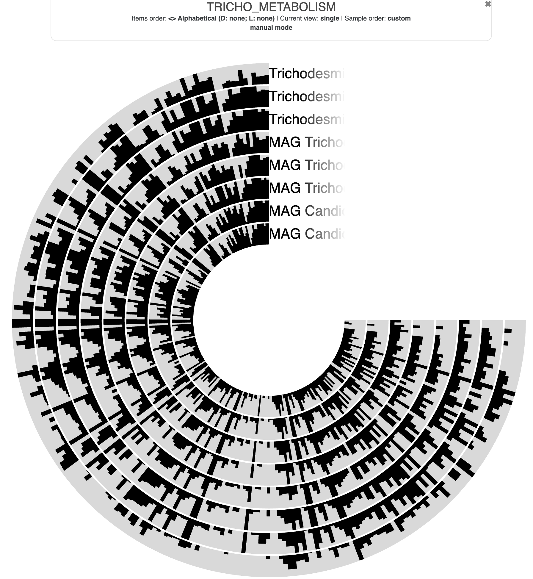
We can make it much easier to see differences between the genomes by doing the following things:
- making the visualization rectangular (and bigger)
- changing the bar plots into a heatmap (‘Intensity’ chart type)
- playing with the Min values to filter out highly incomplete modules
- clustering the genomes so that genomes with similar metabolic capacity are close together
- clustering the modules so that modules with similar distribution across genomes are close together
- importing the name and categories of each module
The first three things can be done by tweaking the interface settings. And if you click on the dropdown box below, you can see all the terminal steps for clustering and importing.
Show/Hide Organizing the metabolism heatmap
Here is how to cluster the modules (rows of the matrix, which become ‘items’ in the interface):
anvi-matrix-to-newick tricho_metabolism-module_pathwise_completeness-MATRIX.txt
This tree file can be given directly to anvi-interactive using the -t parameter. Or, you could import it into the profile-db as an ‘items order’ using the program anvi-import-items-order. We’ll stick to the former in this tutorial.
Here is how to cluster the genomes (columns of the matrix, which become ‘layers’ in the interface). First, you flip the matrix to put the genomes into the rows, and then you use the same anvi-matrix-to-newick command as before:
anvi-script-transpose-matrix tricho_metabolism-module_pathwise_completeness-MATRIX.txt -o tricho_metabolism-module_pathwise_completeness-MATRIX-transposed.txt
anvi-matrix-to-newick tricho_metabolism-module_pathwise_completeness-MATRIX-transposed.txt
Then, you put the resulting dendrogram into a misc-data-layer-orders-txt file:
# read the file into a variable, and then print to a new tab-delimited file
TREE=$(cat tricho_metabolism-module_pathwise_completeness-MATRIX-transposed.txt.newick)
echo -e "item_name\tdata_type\tdata_value\nmag_organization\tnewick\t$TREE" > layer_order.txt
This allows you to import the dendrogram into the profile-db:
anvi-import-misc-data -p metabolism_profile.db -t layer_orders \
                      layer_order.txt
Finally, we want to see module information like names and categories, not just the module numbers. Here’s a little set of SQL queries to extract that information from the modules-db (use the database from the same KEGG data directory you’ve been using all along):
# if you aren't using the default KEGG data dir, you should change this variable to point to the MODULES.db in the dir you ARE using
export ANVIO_MODULES_DB=`python -c "import anvio; import os; print(os.path.join(os.path.dirname(anvio.__file__), 'data/misc/KEGG/MODULES.db'))"`
sqlite3 $ANVIO_MODULES_DB "select module,data_value from modules where data_name='NAME'" | \
    tr '|' '\t' > module_names.txt
sqlite3 $ANVIO_MODULES_DB "select module,data_value from modules where data_name='CLASS'" | \
    tr '|' '\t' > module_categories.txt
You can split the category strings into 3 different columns, and combine everything into one table:
echo -e "class\tcategory\tsubcategory" > category_columns.txt
cut -f 2 module_categories.txt | sed 's/; /\t/g' >> category_columns.txt
echo -e "module\tname" > name_columns.txt
cat module_names.txt >> name_columns.txt
paste name_columns.txt category_columns.txt > module_info.txt
Then you can import that new table into the profile-db:
anvi-import-misc-data -t items -p metabolism_profile.db module_info.txt

## clean up
rm module_names.txt module_categories.txt name_columns.txt category_columns.txt
Now you should have everything you need for visualizing the data nicely.
Once you are finished with the code in the dropdown box, you can visualize the pathwise completeness matrix again like this (adding the module organization with the -t parameter):
anvi-interactive -d tricho_metabolism-module_pathwise_completeness-MATRIX.txt \
                  -p metabolism_profile.db \
                  --manual \
                  --title TRICHO_METABOLISM \
                  -t tricho_metabolism-module_pathwise_completeness-MATRIX.txt.newick
In case you want your visualization to exactly match ours, you can import our settings into the profile-db for the heatmap. Note that the organization will only work if you named your trees the same way we did.
anvi-import-state -s ../00_DATA/metabolism_state.json \
                  -p metabolism_profile.db \
                  -n default
The heatmap should ultimately look something like this:
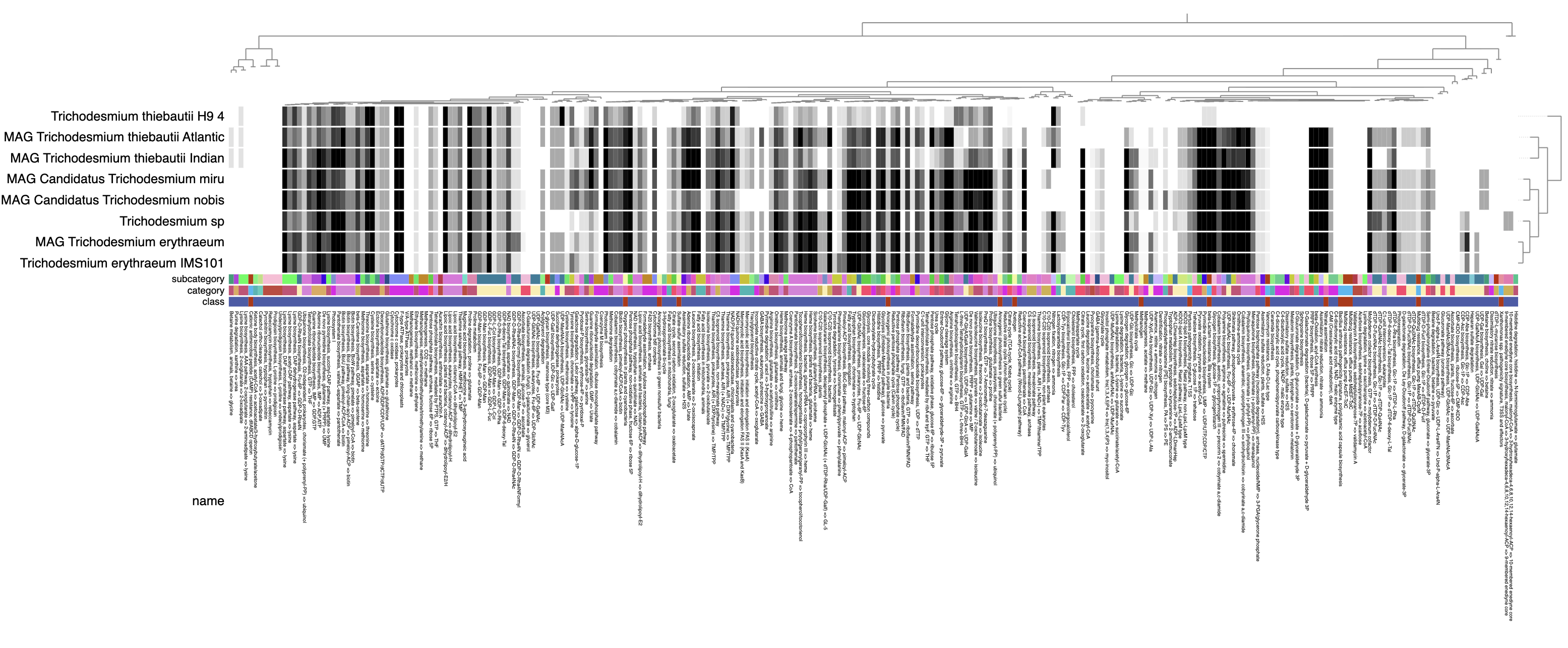
A few things we can notice from the visualization:
- In the genome clustering, there are three main groups of metabolically-similar genomes: all the T. erythraeum genomes are together, all the T. thiebautii genomes are together, and the two candidate species T. miru and T. nobis are together.
- The rather incomplete T. thiebautii H9 genome is clearly missing a lot of metabolic pathways that it shouldn’t actually be missing, particularly on the right side of the heatmap where there are plenty of modules shared by all of the other 7 genomes.
- It should be fairly easy now to spot the modules that are missing specifically in T. miru and T. nobis. Here they are, highlighted in orange:
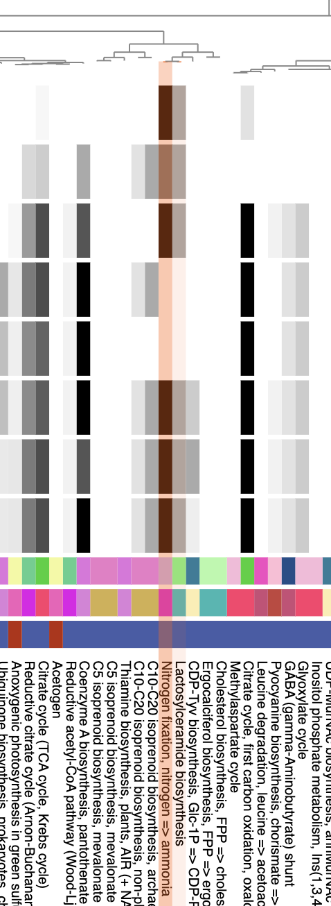
As expected, the nitrogen fixation module is there.
Right next to the nitrogen fixation module is an unusual sounding metabolic pathway, Lactosylceramide biosynthesis, which is 50% complete in all of the other genomes. Lactosylceramides are a type of glycosphingolipid, not very well studied in Cyanobacteria (except for some work investigating sphingolipid roles in plant-microbe symbiotic interactions (Heaver, Johnson and Ley 2018)), so perhaps it is not this exact pathway that is relevant, but rather some of the enzymes in it. Indeed, if you look at the details of M00066 in the long-format output file, you will see that only one enzyme is annotated in these genomes: ceramide glucosyltransferase (K00720). Unfortunately, this enzyme is also not well studied in bacteria, so we don’t have much literature backup for interpreting the lack of this function in T. miru and T. nobis. Maybe a sphingolipid expert will see this one day and look into it. :)
Using custom metabolic modules
When we estimated metabolism with the default KEGG modules in the previous section, a lot of the completeness scores were quite similar across all 8 of our genomes. But we know from Tom’s paper that there are a few other nitrogen fixation-related activities that T. miru and T. nobis do not have and that the other genomes do. The KEGG modules don’t really capture what makes these genomes different. Additionally, the KEGG module for nitrogen fixation isn’t comprehensive (as I mentioned before).
So let’s fix that, by using our own set of custom metabolic modules. There are some in the datapack at 00_DATA/modules/. They include a nitrogen fixation module with the full nif gene set (nifHDK and nifENB), a module for hydrogen recycling (hyaABD and hypABCDEF), a module for hopanoid lipid production (squalene synthase, squalene-hopene cyclase, and hpnABGH), and a module for nitrite/nitrate transport (nark and tauABC). The first three are related to nitrogen fixation and associated metabolic activities, while the last one is related to nitrogen assimilation (an alternative to nitrogen fixation) – hence, we expect to find only the last module complete in T. miru and T. nobis.
Here is the custom module for hopanoid production as an example:
ENTRY       NIF003
NAME        Hopanoid lipid production
DEFINITION  (K00801,COG1562) (K06045,COG1657) PF01370.25 PF00535.30 PF01048.24 PF04055.25+PF11946.12
ORTHOLOGY   K00801   farnesyl-diphosphate farnesyltransferase [EC:2.5.1.21]
            COG1562  phytoene/squalene synthetase
            K06045   squalene-hopene/tetraprenyl-beta-curcumene cyclase [EC:5.4.99.17 4.2.1.129]
            COG1657  terpene cyclase SqhC
            PF01370.25  Hopanoid-associated sugar epimerase HpnA
            PF00535.30  Hopene-associated glycosyltransferase HpnB
            PF01048.24  Putative hopanoid-associated phosphorylase HpnG
            PF04055.25  Hopanoid biosynthesis associated radical SAM protein HpnH (Radical SAM domain)
            PF11946.12  Hopanoid biosynthesis associated radical SAM protein HpnH (unknown associated domain)
CLASS       User modules; Biosynthesis; Lipid biosynthesis
ANNOTATION_SOURCE   K00801  KOfam
                    K06045  KOfam
                    COG1562  COG24_FUNCTION
                    COG1657  COG24_FUNCTION
                    PF01370.25  Pfam
                    PF00535.30  Pfam
                    PF01048.24  Pfam
                    PF04055.25  Pfam
                    PF11946.12  Pfam
///
As you can see, it includes enzymes from multiple annotation sources. We’ve already annotated our genomes with all of those functional databases, so we are good to go.
To set up the custom modules into a modules database that we can use with anvi-estimate-metabolism, we need to use the program anvi-setup-user-modules:
anvi-setup-user-modules -u ../00_DATA/
Doing so creates a database at 00_DATA/USER_MODULES.db containing these four modules. We can now give this database to anvi-estimate-metabolism with the -u parameter. We’ll also use the --only-user-modules flag to skip the KEGG module estimation.
Additionally, we will ask the program to compute module copy numbers for us with the --add-copy-number flag. Copy numbers are usually more suitable for metagenomic input rather than individual genomes, but transporter genes can often occur in multiple copies in a single genome and we want to be able to capture that signal in our estimation output.
anvi-estimate-metabolism -e external-genomes.txt \
            -u ../00_DATA/ \
            --only-user-modules \
            --add-copy-number \
            -O nitrogen_metabolism
Take a look at the output (nitrogen_metabolism_modules.txt). What do you notice?
For convenience, I’ll also show the heatmap of pathway completeness scores and the heatmap of per-step copy numbers:
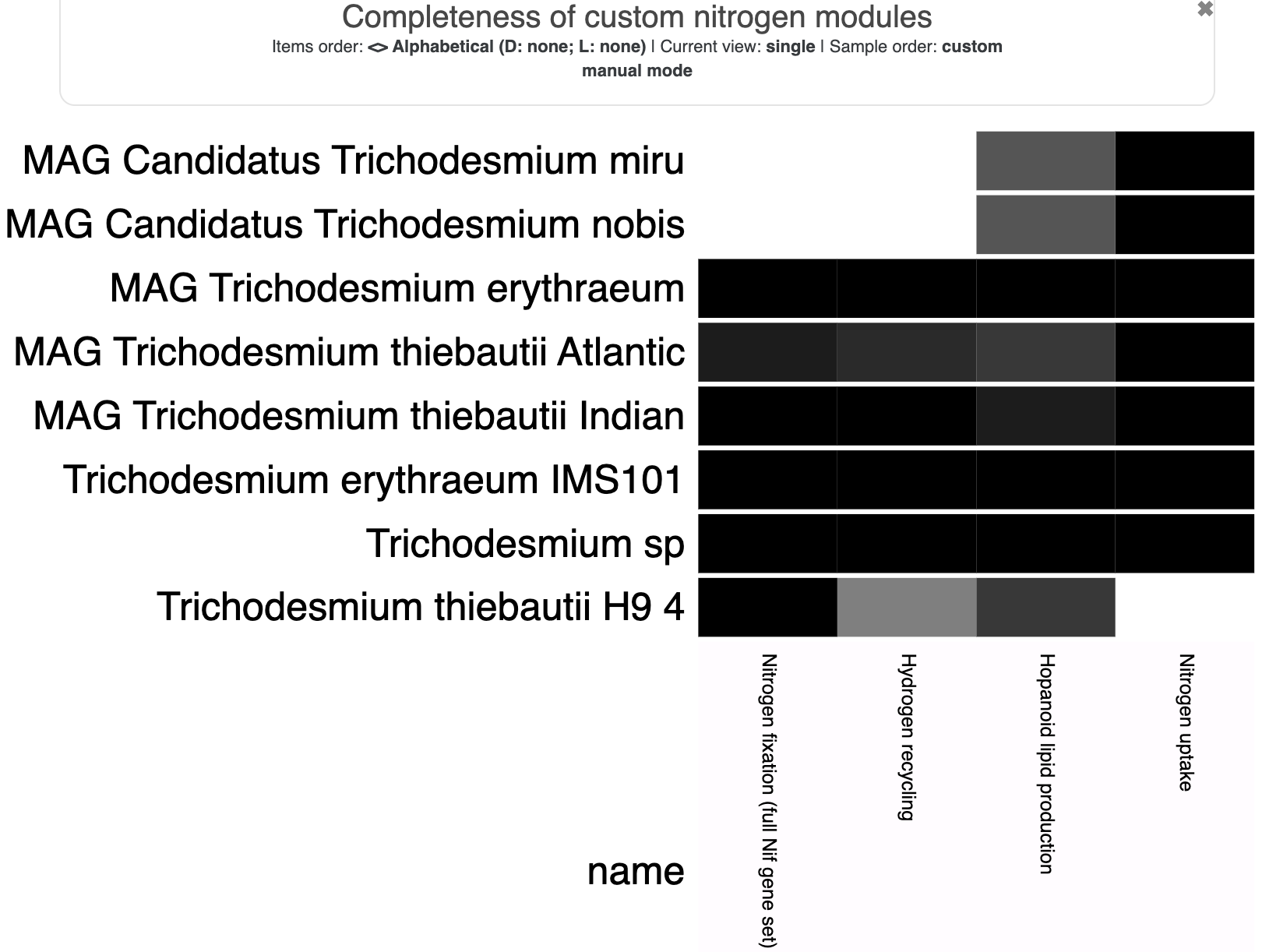
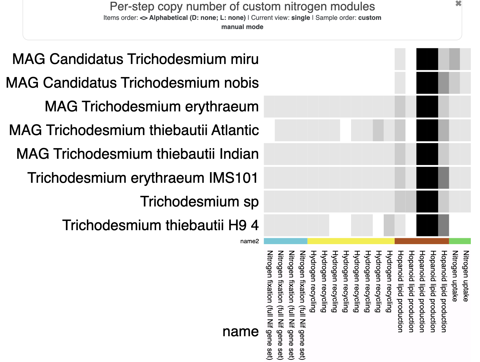
In these visualizations, we’ve adjusted the min/max values to better show the different values. The completeness score heatmap has a minimum of 0.25 (so any completeness value below that appears white) and the normal maximum of 1.0. The copy number heatmap has the normal minimum of 0 and a maximum of 10 (so any copy number above 10 appears black) – there are some steps that have way more than 10 copies, which makes the typical range of 0-2 copies extremely difficult to see on the heatmap unless we cap the value.
Show/Hide Commands to generate the heatmaps
Just like before, if you want a heatmap, you’ll have to generate the output in matrix format:
anvi-estimate-metabolism -e external-genomes.txt \
            -u ../00_DATA/ \
            --only-user-modules \
            --add-copy-number \
            -O nitrogen_metabolism \
            --matrix-format
For a heatmap this small, we don’t really need to cluster anything. But it would be nice to see the module names instead of just their numbers, so we’ll make a little table of names:
echo -e "module\tname" > custom_mod_names.txt
sqlite3 ../00_DATA/USER_MODULES.db "select module,data_value from modules where data_name='NAME'" | \
        tr '|' '\t'  >> custom_mod_names.txt
Since we need a profile database before we can store any additional data in it, we’ll go ahead and run anvi-interactive with the --dry-run flag to create one. Then we can import the module name data. If you want, you can also import a state file to automatically make the visualization into a heatmap.
anvi-interactive -d nitrogen_metabolism-module_pathwise_completeness-MATRIX.txt \
                  -p nitrogen_completeness.db \
                  --manual \
                  --title "Completeness of custom nitrogen modules" \
                  --dry-run

anvi-import-misc-data -p nitrogen_completeness.db -t items custom_mod_names.txt

# if you want, import the heatmap visualization settings
anvi-import-state -p nitrogen_completeness.db -n default -s ../00_DATA/nitrogen_heatmap.json
Finally, here is the visualization command (this time without --dry-run):
anvi-interactive -d nitrogen_metabolism-module_pathwise_completeness-MATRIX.txt \
                  -p nitrogen_completeness.db \
                  --manual \
                  --title "Completeness of custom nitrogen modules"
If you also want to make the per-step copy number heatmap, it is a similar chain of commands. The only difference is the module name info file, which now has to be based on the step names. Here are all the commands to run:
# a little BASH loop to generate the step names file
# with a little trick: two columns for the name so that one can be colors and one can be text
echo -e "step\tname\tname2" > custom_step_names.txt
while read step; do \
  mod=$(echo $step | cut -d '_' -f 1); \
  name=$(grep $mod custom_mod_names.txt | cut -f 2); \
  echo -e "$step\t$name\t$name" >> custom_step_names.txt; \
done < <(cut -f 1 nitrogen_metabolism-step_copy_number-MATRIX.txt | tail -n+2)

# get a profile db
anvi-interactive -d nitrogen_metabolism-step_copy_number-MATRIX.txt \
                  -p nitrogen_step_copies.db \
                  --manual \
                  --title "Per-step copy number of custom nitrogen modules" \
                  --dry-run

# import relevant data
anvi-import-misc-data -p nitrogen_step_copies.db -t items custom_step_names.txt
anvi-import-state -p nitrogen_step_copies.db -n default -s ../00_DATA/nitrogen_step_copies.json

# visualize
anvi-interactive -d nitrogen_metabolism-step_copy_number-MATRIX.txt \
                  -p nitrogen_step_copies.db \
                  --manual \
                  --title "Per-step copy number of custom nitrogen modules"
Here are some of my observations:
- As we expected, T. miru and T. nobis only have the
NIF004(Nitrogen uptake) module complete. - The other 6 genomes have all the modules >80% complete (except for H9, which is missing several genes from the hydrogen recycling and nitrogen uptake modules. But we already know it is quite an incomplete genome).
- T. miru and T. nobis have multiple copies of the narK transporter (as Tom found in his paper) while the others each have one. This isn’t enough to make the overall nitrogen uptake module have a higher copy number, but you can see the copies of the individual transporters in the last column (
per_step_copy_numbers), and in the copy number heatmap. - Interestingly, the hopanoid lipid production module (
NIF003) has relatively high completeness in most genomes (including T. miru and T. nobis, in which the module is 75% complete), and a lot of that seems to result from finding many Pfam annotations for the hpn gene domains. This contrasts with the results from Tom’s paper – Tom used the RAST annotation tool to find the hpnABGH genes, which may have been a more stringent and/or specific strategy. Perhaps these Pfam domains are too generic to indicate hopanoid production? If we were serious about this analysis, we would probably cross-check our module with a lipid biosynthesis expert to make sure it is appropriate for identifying this metabolic capacity. :) - One thing looks weird! If you look at the per-step copy numbers for
NIF003, the last step always has a copy number of 0 – even though there are certainly genomes in which both hpnH Pfam domains are annotated. In fact, for 6 of the genomes, the pathwise copy number is 1 (or 2) while the stepwise copy number is 0.
Let’s look into that last point a bit more. What is going with the stepwise copy number estimation for hopanoid production? When things look weird in the results, it is always good to take a single genome, rerun the metabolism estimation, and pay attention to the warnings in the terminal output. Terminal output is more verbose on individual genomes than in ‘multi-mode’ for anvi-estimate-metabolism.
The T. erythraeum genome shows this weird copy number pattern, so let’s use that one:
anvi-estimate-metabolism -c ../Trichodesmium_erythraeum_IMS101-contigs.db \
                  -u ../00_DATA/ \
                  --only-user-modules \
                  -O test \
                  --add-copy-number
Aha! There is a relevant warning in the terminal output:
WARNING
===============================================
The gene call 208 has multiple annotations to alternative enzymes within the
same step of a metabolic pathway (PF04055.25, PF11946.12), and these enzymes
unfortunately have a complex relationship. The affected module is NIF003, and
here is the step in question: PF04055.25+PF11946.12. We arbitrarily kept only
one of the annotations to this gene in order to avoid inflating the step's copy
number, but due to the complex relationship between these alternatives, this
could mean that the copy number for this step is actually too low. Please heed
this warning and double check the stepwise copy number results for NIF003 and
other pathways containing gene call 208.
The lessons here: pay attention to warnings from anvi’o programs. And keep in mind that many of these warnings are suppressed when processing multiple inputs, so testing things on individual genomes might be the way to go when outputs look strange.
If something goes wrong (or weird) while using anvi’o, you may want to try re-running whatever you just did with the addition of the global --debug flag (which works for all anvi’o programs). This flag enables extra terminal output, which in the best case may help you figure out what is going on, and in the worst case can provide enough information to send to the developers when you ask them for help (in case of errors, we especially appreciate the code tracebacks that --debug allows you to see).
If you found this section useful and you want to make your own custom metabolic modules, check out this guide on the user-modules-data help page.
Reaction networks and drawing KEGG Pathway Maps
Let’s move onto the second type of metabolism reconstruction: metabolic modeling. Anvi’o can generate a reaction-network from the KEGG Ortholog (KO) annotations in any contigs database or pangenome database. The network connects all genes with KO annotations to the chemical reactions they catalyze, and the metabolites consumed or produced by those reactions. Reaction and compound information are taken from the ModelSEED database.
If you want to use these programs, you will first have to run anvi-setup-modelseed-database (if you haven’t already done so in your anvi’o environment).
Let’s make a reaction network for one genome using the program anvi-reaction-network:
anvi-reaction-network -c ../Trichodesmium_sp-contigs.db
There will be plenty of output on your terminal screen, but no output files added to your working directory – the network will be stored directly in the contigs database.
Now, if you wanted to do some flux balance analysis (FBA) to model the flow of metabolites through this network – bad news, you can’t do that (at least, not yet) in anvi’o. However, you can export the reaction-network into a JSON file suitable for common metabolic modeling software (like COBRApy) with the program anvi-get-metabolic-model-file:
anvi-get-metabolic-model-file -c ../Trichodesmium_sp-contigs.db \
                -o Trichodesmium_sp_rxn_network.json
The output file is really big, because it contains every single metabolite, reaction, and gene contributing to the reaction network.
What we will do in anvi’o is to use this reaction-network for some neat visualizations of KEGG Pathway Maps with the program anvi-draw-kegg-pathways.
anvi-draw-kegg-pathways --contigs-dbs ../Trichodesmium_sp-contigs.db \
              -o Trichodesmium_sp_PATHWAY_MAPS \
              --ko
For each KEGG Pathway Map, the program will highlight the KOs from the map that are annotated in each provided genome, and create a PDF file in the specified output directory. We only provided a single genome, so the resulting maps are specific to that genome’s annotations.
Let’s look at an example map. Of course we will look at the Nitrogen Metabolism map (which is map 00910 and stored at Trichodesmium_sp_PATHWAY_MAPS/kos_00910.pdf):
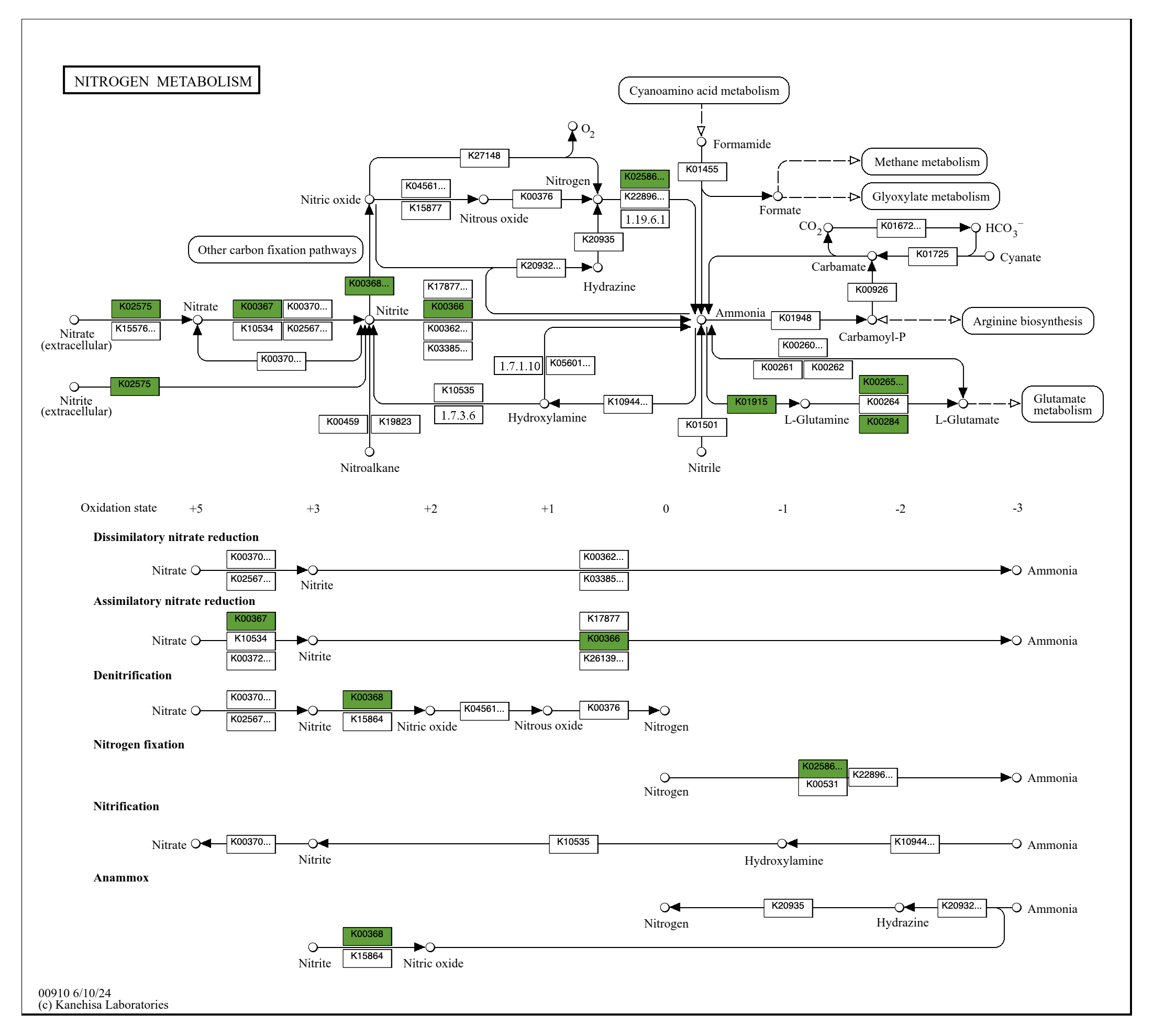
You can see that in addition to nitrogen fixation (nitrogen to ammonia), this microbe can also import nitrate and nitrate from the extracellular matrix into the cell, convert nitrate to nitrite (assimilatory nitrate reduction) and to nitric oxide, convert nitrite to ammonia, and feed that ammonia into glutamate metabolism – which is the start of amino acid biosynthesis using that fresh new bioavailable nitrogen.
While pathway prediction gives you quantitative summaries of metabolic capacity, these Pathway Map drawings are great for understanding what is actually going on in those pathways, and for seeing the connections between different classes of metabolism. Each map gives you an overall picture of a small-ish, digestible and ecologically-relevant part of the entire reaction network.
I bet you are wondering how this map looks different across our Trichodesmium genomes. If so, then you are in luck, because we can also use anvi-draw-kegg-pathways to compare metabolic capacity of multiple genomes.
First, we will need to run anvi-reaction-network on all the other genomes. This program unfortunately doesn’t accept an external genomes file as input; however, we can reuse our BASH loop strategy from above.
while read genome
do
    anvi-reaction-network -c ../${genome}-contigs.db; \
done < ../genomes.txt
Once that is done, we can run anvi-draw-kegg-pathways again, and this time we can provide an external genomes file. We will also provide the --draw-grid flag so that we get maps showing the results from each individual genome (in addition to the default map showing the total annotations across all genomes). Since it would take a long time to draw every single Pathway Map for all 8 genomes, we will focus on a subset of maps as specified by the --pathway-numbers parameter – the list below includes a couple of maps related to nitrogen metabolism, a few for photosynthesis and related metabolic capacities, and a map for metabolism of some amino acids.
anvi-draw-kegg-pathways --external-genomes ../external-genomes.txt \
                -o ALL_PATHWAY_MAPS \
                --ko \
                --draw-grid \
                --pathway-numbers 00910 01310 00195 00860 00906 00900 00260 00290
The resulting files in the ALL_PATHWAY_MAPS include:
- multiple map
.pdffiles (one per requested Pathway Map) with colored boxes showing the number of annotations to a given KO across all input genomes - a
colorbar.pdfshowing the legend – what color corresponds to what count - a
grid/subdirectory containing similarly-named map.pdffiles, except this time each one shows a grid of individual maps for each genome
For consistency with above, we’ll look at Pathway Map 00910 for Nitrogen Metabolism again. Here is the combined map at ALL_PATHWAY_MAPS/kos_00910.pdf:
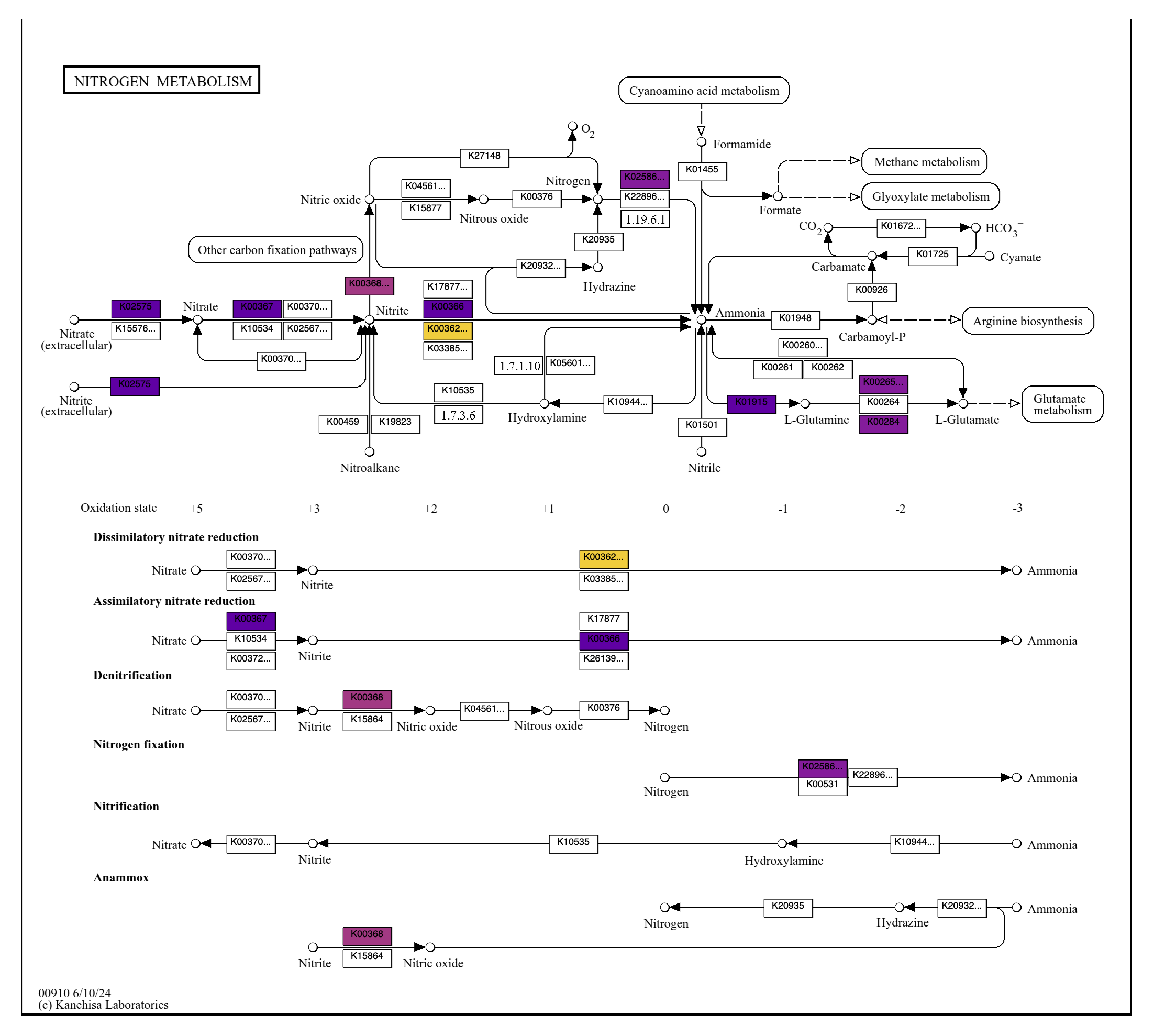
The legend tell us that smaller counts are warm colors (starting from a count of 1 in yellow) and higher counts are warm colors (going to a max of 8 in dark purple). So we can tell from this map that all the genomes encode enzymes for assimilatory nitrate reduction, 6 out of the 8 genomes encode nitrogen fixation, and only 1 genome can convert nitrite to ammonia. But we don’t know which genome can do what.
To reveal the specific distribution of enzymes across genomes, here is the corresponding grid map (ALL_PATHWAY_MAPS/grid/kos_00910.pdf):
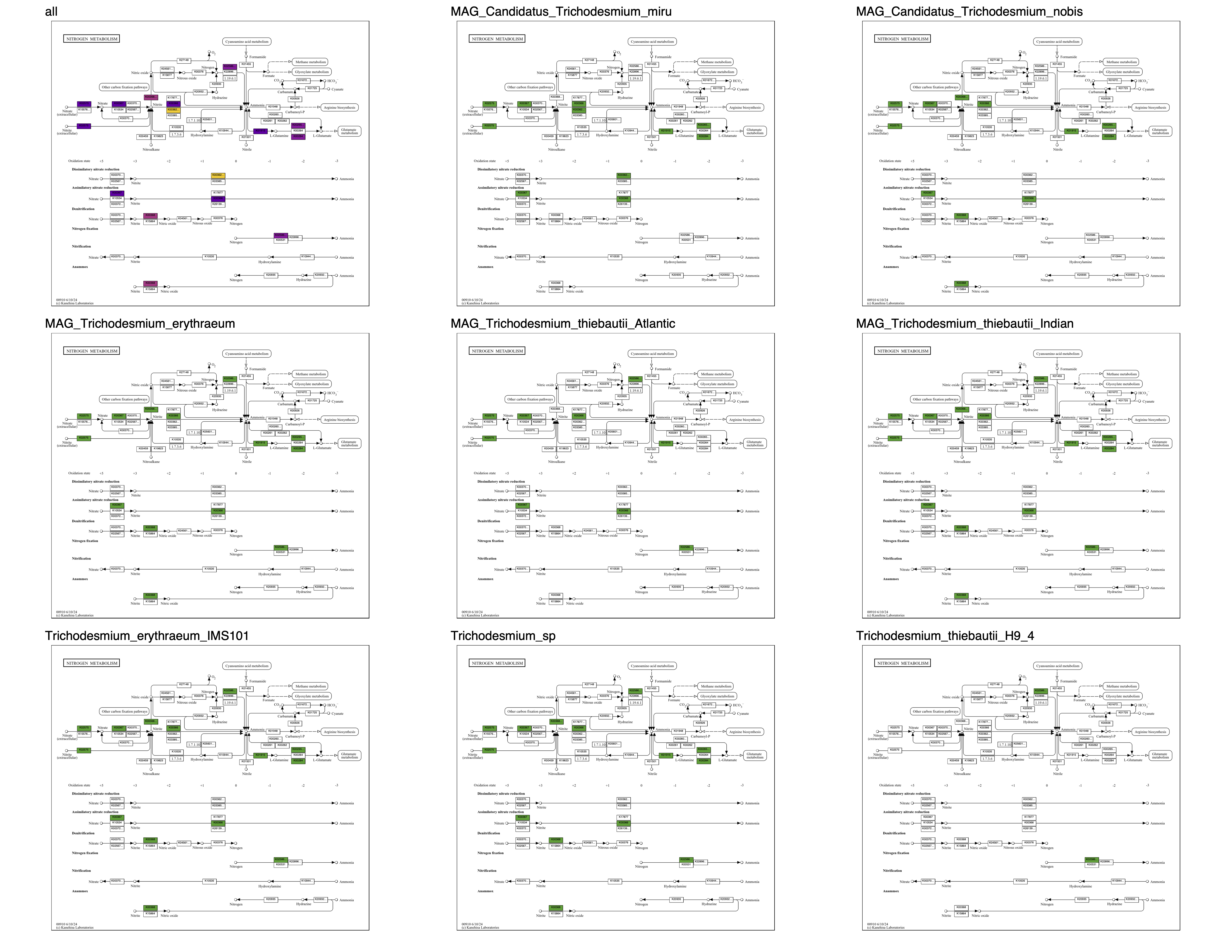
Now it is clear that T. miru and T. nobis are missing nitrogen fixation (as we know), and that T. miru is the only species that can convert nitrite to ammonia.
I encourage you to look through the other maps (both overall and in grid form). Here are some things to look out for:
- The nitrogen cycle map (01310) shows metabolic capacity with colored reaction arrows rather than boxes. There again you can see that T. miru is the only one doing nitrogen dissimilation.
- In map 00260 (Glycine, Serine and Threonine Metabolism), you can see that T. miru and T. nobis are also the only genomes with the enzyme to convert threonine to 2-oxobutanoate (a precursor leading into the production of several other amino acids). You can see the same thing in map 00290 (Valine, Leucine and Isoleucine Biosynthesis). Clearly the other genomes have the capacity to make those amino acids, just not by starting from 2-oxobutanoate. So biosynthesis of amino acids is just a bit more connected in T. miru and T. nobis compared to the others.
- Map 00195 shows photosynthesis. Maps 00860, 00900, and 00906 are photosynthesis-related capacities, like the biosynthesis of pigments. These are things that all the Trichodesmium species can do, but there are still differences between these genomes – some genomes are missing enzymes that all the others have (a detection issue?) while others have some enzymes that all the others don’t (interesting ecology?).
The KEGG Pathway Maps cover many metabolic capacities that KEGG modules do not, and can be a great tool for comparative metabolism analyses.
Predicting metabolic interactions
One cool thing about Trichodesmium is that they have friends. Bacterial friends, to be specific. Trichodesmium colonies harbor associated bacteria like Alteromonas, Roseibium, and Balneolales species. Based on a recent study about a Red Sea T. thiebautii colony and its bacterial associates Koedooder et al 2023, these microbes have a symbiotic relationship – they help each other by exchanging important molecules. The bacterial associates are known to produce siderophores, which help with harvesting iron from dust in their environment and which Trichodesmium cannot make itself. Meanwhile, Trichodesmium can make several B vitamins that the bacterial associates are auxotrophic for.
Wouldn’t it be cool if we could investigate metabolic interactions using our genomes, without having to painstakingly search for individual gene annotations? Anvi’o got u, fam.
There is a program called anvi-predict-metabolic-exchanges that leverages the reaction-network infrastructure to identify potential metabolites that could be exchanged between two microbes from their genomic data. It does so by examining the reactions in the network to find metabolites that could be produced by only one of the organisms and consumed by the other. If possible, it then leverages the KEGG Pathway Maps that we saw in the previous section to walk over targeted subsets of the network starting from the potential exchange point, in order to compute statistics about the reaction chains leading up to (or away from) the exchange. Those statistics – length, amount of overlap between genomes, etc – serve as evidence for the likelihood of a potential exchange. The program also identifies which compounds are uniquely produced or consumed by one of the genomes in the pair. You can find more technical information about how anvi-predict-metabolic-exchanges works here.
anvi-predict-metabolic-exchanges is an extremely new program as of October 2025. It is not fully refined yet and there may be some remaining bugs. Please validate the results carefully and report issues if you notice weird results. The developers thank you for your patience :)
We are going to test this program out on our T. thiebautii (Atlantic) genome and three genomes of known associated bacteria based on the Koedooder et al 2023 study. The MAGs from that study are not yet publicly available, so instead we will work with reference genomes – one for Alteromonas macleodii (GCF_002849875.1), one for Roseibium aggregatum (GCF_000168975.1), and one for Marinobacter salarius (GCF_002116735.1).
You’ve already learned how to do all the preparatory steps for analyzing genomes – making a contigs database, annotating with KOfams, and creating the reaction network. Feel free to practice on these three new genomes. But in case you just want to get right to the metabolic interactions analysis, there are pre-made, annotated contigs databases for these genomes in the datapack at 00_DATA/associate_dbs/.
You can copy the databases over to your current working directory (assuming you are still in the 02_METABOLISM folder) like so:
cp ../00_DATA/associate_dbs/*.db .
For those interested, click the Show/Hide box below to see how we made those databases.
Show/Hide Steps to make the contigs databases
# download and reformat
curl https://ftp.ncbi.nlm.nih.gov/genomes/all/GCF/002/849/875/GCF_002849875.1_ASM284987v1/GCF_002849875.1_ASM284987v1_genomic.fna.gz -o GCF_002849875.1_ASM284987v1_genomic.fna.gz
gunzip GCF_002849875.1_ASM284987v1_genomic.fna.gz
anvi-script-reformat-fasta GCF_002849875.1_ASM284987v1_genomic.fna -o A_macleodii.fasta --simplify-names --prefix GCF_002849875 --seq-type NT
curl https://ftp.ncbi.nlm.nih.gov/genomes/all/GCF/000/168/975/GCF_000168975.1_ASM16897v1/GCF_000168975.1_ASM16897v1_genomic.fna.gz -o GCF_000168975.1_ASM16897v1_genomic.fna.gz
gunzip GCF_000168975.1_ASM16897v1_genomic.fna.gz
anvi-script-reformat-fasta GCF_000168975.1_ASM16897v1_genomic.fna -o R_aggregatum.fasta --simplify-names --prefix GCF_000168975 --seq-type NT
curl https://ftp.ncbi.nlm.nih.gov/genomes/all/GCF/002/116/735/GCF_002116735.1_ASM211673v1/GCF_002116735.1_ASM211673v1_genomic.fna.gz -o GCF_002116735.1_ASM211673v1_genomic.fna.gz
gunzip GCF_002116735.1_ASM211673v1_genomic.fna.gz
anvi-script-reformat-fasta GCF_002116735.1_ASM211673v1_genomic.fna -o M_salarius.fasta --simplify-names --prefix GCF_002116735 --seq-type NT
rm GCF_00*.fna

# make contigs databases
for g in A_macleodii R_aggregatum M_salarius; do
  anvi-gen-contigs-database -f $g.fasta -o $g-contigs.db -T 3
done

# annotate with KOfams
for g in A_macleodii R_aggregatum M_salarius; do
  anvi-run-kegg-kofams -c $g-contigs.db -T 4;
done

# make reaction network
for g in A_macleodii R_aggregatum M_salarius; do
  anvi-reaction-network -c $g-contigs.db;
done
Since the databases have reaction networks already stored inside them, we can get right to predicting interactions. Let’s start by running anvi-predict-metabolic-exchanges on one pair of genomes:
anvi-predict-metabolic-exchanges -c1 ../MAG_Trichodesmium_thiebautii_Atlantic-contigs.db \
                -c2 A_macleodii-contigs.db \
                -O thiebautii-vs-macleodii \
                -T 4
There were probably some warnings on your screen about some Pathway Maps not having a “reaction (RN) type KGML file”. This just means that we couldn’t use those specific Maps when doing the Pathway Map walks for computing evidence. If you don’t want to see the warnings, you can specifically exclude the missing Maps with the flag --exclude-pathway-maps (we will do this later).
There are actually two prediction strategies used by anvi-predict-metabolic-exchanges, and the terminal output will tell you how many predictions were made using each one. Briefly, the first strategy (“Pathway Map Walk”) is based on the KEGG Pathway Maps – it works on only a subset of metabolites, but it generates high-quality predictions that are associated with evidence from the Pathway Map walks. The second strategy (“Reaction Network Subset”) works on all metabolites in the network (even those not in KEGG Pathway Maps), but generates predictions that are potentially less accurate. That distinction is reflected in the sheer number of predictions that we get from either approach:
Number of exchanged compounds predicted from KEGG Pathway Map walks : 125
Number of unique compounds predicted from KEGG Pathway Map walks : 621
(...)
Number of exchanged compounds predicted from Reaction Network subset approach : 309
Number of unique compounds predicted from Reaction Network subset approach : 1,341
The Pathway Map walk approach gives you fewer predictions, while the reaction network subset approach gives you more (but lower confidence) predictions. Note that you can turn off either approach by using the --no-pathway-walk or --pathway-walk-only flags, respectively.
Here is the summary of the results from the terminal:
OVERALL RESULTS
===============================================
Identified 434 potentially exchanged compounds and 1962 compounds unique to one
genome.
These results are described in three output files: thiebautii-vs-macleodii-potentially-exchanged-compounds.txt describes the potential exchanges (with summaries of the evidence from associated Pathway Maps), thiebautii-vs-macleodii-evidence.txt contains the full set of statistics from all Pathway Map walks, and thiebautii-vs-macleodii-unique-compounds.txt describes the metabolites that are uniquely produced or consumed by one of the organisms. All of these output files are indexed by ModelSEED compound ID numbers.
Our predictions are limited to the metabolites we can find in the ModelSEED database. ModelSEED doesn’t contain compounds for siderophores like petrobactin, vibrioferrin, or agrobactin. So we cannot find those specific interactions as described in the Koedooder et al 2023 paper.
But we might be able to find the B vitamin exchanges mentioned in that paper, or perhaps something new! Let’s take a careful look at the predicted exchanges. Here are the first 10 lines of that file:
compound_id |
compound_name |
genomes |
produced_by |
consumed_by |
prediction_method |
max_reaction_chain_length |
max_production_chain_length |
production_overlap_length |
production_overlap_proportion |
production_chain_pathway_map |
max_consumption_chain_length |
consumption_overlap_length |
consumption_overlap_proportion |
consumption_chain_pathway_map |
|---|---|---|---|---|---|---|---|---|---|---|---|---|---|---|
| cpd00027 | D-Glucose | A_macleodii,MAG_Trichodesmium_thiebautii_Atlantic | A_macleodii | MAG_Trichodesmium_thiebautii_Atlantic | Pathway_Map_Walk | 10 | 8 | None | None | 00500 | 2 | 2 | 1.0 | 00500 |
| cpd00037 | UDP-N-acetylglucosamine | A_macleodii,MAG_Trichodesmium_thiebautii_Atlantic | A_macleodii | MAG_Trichodesmium_thiebautii_Atlantic | Pathway_Map_Walk | 14 | 6 | None | None | 00520 | 8 | 8 | 1.0 | 00550 |
| cpd00044 | 3-phosphoadenylylsulfate | A_macleodii,MAG_Trichodesmium_thiebautii_Atlantic | A_macleodii | MAG_Trichodesmium_thiebautii_Atlantic | Pathway_Map_Walk | 7 | 4 | None | None | 00920 | 3 | 3 | 1.0 | 00920 |
| cpd00065 | L-Tryptophan | A_macleodii,MAG_Trichodesmium_thiebautii_Atlantic | A_macleodii | MAG_Trichodesmium_thiebautii_Atlantic | Pathway_Map_Walk | 14 | 13 | None | None | 00400 | 1 | 1 | 1.0 | 00380 |
| cpd00085 | beta-Alanine | MAG_Trichodesmium_thiebautii_Atlantic,A_macleodii | MAG_Trichodesmium_thiebautii_Atlantic | A_macleodii | Pathway_Map_Walk | 10 | 1 | None | None | 00410,00770 | 9 | 2 | 0.2222222222222222 | 00770 |
| cpd00098 | Choline | MAG_Trichodesmium_thiebautii_Atlantic,A_macleodii | MAG_Trichodesmium_thiebautii_Atlantic | A_macleodii | Pathway_Map_Walk | 3 | 1 | 1 | 1.0 | 00564 | 2 | None | None | 00260 |
| cpd00100 | Glycerol | A_macleodii,MAG_Trichodesmium_thiebautii_Atlantic | A_macleodii | MAG_Trichodesmium_thiebautii_Atlantic | Pathway_Map_Walk | 2 | 1 | None | None | 00052,00561 | 1 | 1 | 1.0 | 00561 |
| cpd00104 | BIOT | MAG_Trichodesmium_thiebautii_Atlantic,A_macleodii | MAG_Trichodesmium_thiebautii_Atlantic | A_macleodii | Pathway_Map_Walk | 5 | 2 | 2 | 1.0 | 00780 | 3 | None | None | 00780 |
| cpd00107 | L-Leucine | A_macleodii,MAG_Trichodesmium_thiebautii_Atlantic | A_macleodii | MAG_Trichodesmium_thiebautii_Atlantic | Pathway_Map_Walk | 11 | 10 | None | None | 00290 | 1 | 1 | 1.0 | 00970 |
The predictions are ranked in order from best evidence to no evidence, so all of these at the top are coming from the Pathway_Map_Walk prediction strategy. And here already is one of our expected exchanges: the compound called ‘BIOT’ is actually biotin aka Vitamin B7, and T. thiebautii is potentially cross-feeding it to A. macleodii as suggested in the Koedooder et al 2023 paper.
There are also a few unexpected predictions that look interesting: A. macleodii seems to be able to produce D-glucose, L-Tryptophan, and L-Leucine while T. thiebautii only can consume these compounds. The relatively long production chain lengths indicate that these aren’t isolated production reactions in the network; they are rather part of a longer metabolic pathway. Meanwhile, the None values for the production overlap mean that the T. thiebautii genome doesn’t contain any of the enzymes in the production-associated Pathway Map. In the case of L-Tryptophan, that map is 00400. Let’s check the associated evidence for L-Tryptophan in map 00400 in the evidence file:
compound |
compound_name |
longest_chain_compound_names |
longest_chain_compounds |
longest_chain_reactions |
longest_reaction_chain_length |
maximum_overlap |
organism |
pathway_map |
proportion_overlap |
type |
|---|---|---|---|---|---|---|---|---|---|---|
| cpd00065 | L-Tryptophan | L-Tryptophan,indol,Indoleglycerol phosphate,1-(2-carboxyphenylamino)-1-deoxyribulose 5-phosphate,N-5-phosphoribosyl-anthranilate,Anthranilate,Chorismate,5-O–1-Carboxyvinyl-3-phosphoshikimate,3-phosphoshikimate,Shikimate,3-Dehydroshikimate,5-Dehydroquinate,DAHP,Phosphoenolpyruvate | C00078,C00463,C03506,C01302,C04302,C00108,C00251,C01269,C03175,C00493,C02637,C00944,C04691,C00074 | rn:R00674,rn:R02340,rn:R03508,rn:R03509,rn:R01073,rn:R00985 rn:R00986,rn:R01714,rn:R03460,rn:R02412,rn:R02413,rn:R03084,rn:R03083,rn:R01826 | 13 | None | A_macleodii | 00400 | None | production |
| cpd00065 | L-Tryptophan | None | None | None | None | None | MAG_Trichodesmium_thiebautii_Atlantic | 00400 | None | consumption |
Okay, so far it looks pretty promising. There is a very long chain of reactions to produce tryptophan from phosphoenolpyruvate in A. macleodii, and nothing at all in T. thiebautii. But just to be sure, let’s also visualize map 00400 for these two genomes with anvi-draw-kegg-pathways (and while we are at it, let’s include the production maps for the other two interesting predictions):
anvi-draw-kegg-pathways --contigs-dbs ../MAG_Trichodesmium_thiebautii_Atlantic-contigs.db A_macleodii-contigs.db \
              -o thiebautii-vs-macleodii_PATHWAY_MAPS \
              --pathway-numbers 00400 00500 00290 \
              --draw-grid \
              --ko
Here is the part of that map where tryptophan is produced:
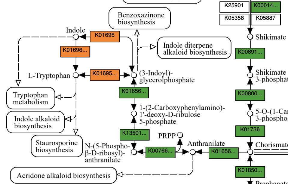
Oh, wait. Only one of the two genomes (A. macleodii) has the enzymes to convert between indole or indoyl-containing compounds and tryptophan, but clearly both genomes have all the rest of the enzymes leading up to that point (we didn’t detect this in T. thiebautii because the start of the reaction chain was missing in its genome). This could be a legitimate gap in T. thiebautii’s reaction network. Or, we could just be missing the annotation for these functions in T. thiebautii (i.e., either we are missing the relevant chunk of the genome, or we failed to annotate the corresponding gene that is present in the MAG).
Perhaps this is a valid exchange, and perhaps it is not. It would take a bit more digging through the T. thiebautii MAG to see if we could find the relevant enzymes (e.g., K01695) with a more careful homology search. But proving that an enzyme is truly missing is hard, and we don’t necessarily want to do that right now. So we are just going to move on.
I encourage you to take a look at the corresponding maps for the production of L-Leucine and D-Glucose. The L-Leucine situation (in map 00290) looks very similar to the L-Tryptophan situation – most of the enzymes are there in both genomes, but T. thiebautii is missing just the tail end of the reaction chain such that it looks like this microbe cannot fully synthesize several amino acids, including leucine, valine and isoleucine. Based on our previous exploration of this pathway map across all of the Trichodesmium genomes, this seems unlikely to be the true story. Most of the other genomes have those enzymes, including the T. thiebautii MAG from the Indian Ocean. So we can ignore this prediction.
For D-Glucose (map 00500), on the other hand, there are many enzymes in the reaction chain that A. macleodii has but T. thiebautii does not. So that prediction looks legitimate – A. macleodii could be cross-feeding glucose to T. thiebautii. Whether or not that actually happens in real life is uncertain. First, A. macleodii would have to intentially create glucose (as opposed to funneling its energy and carbon into other things). Second, it would have to produce more glucose than it individually needs, and third, that glucose would have to make its way outside of the cell where T. thiebautii could pick it up. But this potential exchange of glucose is now a hypothesis that is testable either by experimental means or literature review.
Allowing for gaps in reaction chains
You might be wondering if there is a way to change the stringency of the Pathway Map walks so that they can handle small gaps. Indeed there is! We can set the --maximum-gaps parameter to allow for some number of gaps in the reaction chains. Unfortunately, this won’t fix the case of L-Tryptophan or L-Leucine, because the gap occurs right at the start of the reaction chain and you cannot build a chain that starts from nothing (Iva and Sam need to think about how to get around this edge case). However, it could help create a better ranking for other ambiguous cases in which the gaps are internal to the reaction chain.
So let’s run the predictions again – this time allowing for a gap of 1 missing enzyme. We will also exclude those problematic pathway maps that gave us pesky warnings before. While creating the tutorial, I noticed that allowing for a gap of 1 causes problems with the Pathway Walk on a specific map, 00061 (Fatty acid biosynthesis) – processing that map takes forever, potentially because the gap causes a cycle that the codebase can’t handle quite yet. To avoid the long (potentially infinite) runtime, we will also exclude this specific map.
How did I figure out that map 00061 was the problematic one? I re-ran the program with the --debug flag to get more verbose output, and noticed that map 00061 was the only one that started processing but didn’t finish.
In addition, since we’ve been seeing amino acids in the prediction output, we will add the --use-equivalent-amino-acids flag to make sure that we are considering metabolites like “Lysine” and “L-Lysine” to be the same (which could affect our results). Here is the full command:
anvi-predict-metabolic-exchanges -c1 ../MAG_Trichodesmium_thiebautii_Atlantic-contigs.db \
                -c2 A_macleodii-contigs.db \
                -O thiebautii-vs-macleodii-gap1 \
                --maximum-gaps 1 \
                --use-equivalent-amino-acids \
                --exclude-pathway-maps 00061,00121,00190,00195,00196,00511,00542,00543 \
                -T 4
This time, the number of predictions from the Pathway Map walk approach is a little bit smaller (122 predictions, compared to 125 from before). Some predictions likely went away because we excluded an additional Pathway Map. But the top-ranked results in the table above mostly didn’t change, except for some of the reaction chains getting a bit longer.
So now is the time to do some targeted searches through the rest of the file. You can look through the rest of the predictions using whatever strategy you think is best. I would recommend focusing on our first set of outputs (the ones made without considering gaps), as those are more stringent and seem to be more reliable predictions overall.
Confused by the ModelSEED compound names? You are not a biochemist and are overwhelmed with all this molecular information? Us, too. One option for you is to take the output, pick out the predictions that you have high-confidence in, and give that list to a large-language model (LLM) so it can pick out the ones that are likely to be biologically-relevant in your system. Then you can focus your efforts on carefully validating those predictions.
Here are some of the interesting predictions that I found:
- Nitrate (cpd00209), produced by A. macleodii and consumed by T. thiebautii. You might remember from our earlier exploration of Pathway Map 00910 that T. thiebautii has the enzymes to import extracellular nitrate and convert it to nitrite. Perhaps some of that exterior nitrate is coming from its associated bacteria.
- Thymine (cpd00151) or Thymidine (cpd00184), produced by T. thiebautii and consumed by A. macleodii. These are part of ‘T’ nucleotides and are needed by both organisms. Other marine microbes are known to exchange nucleotide components, so perhaps these do, too.
- Propionate (cpd00141), produced by T. thiebautii and consumed by A. macleodii. This one is interesting because T. thiebautii can produce it but doesn’t seem to be able to use it at all. Meanwhile, A. macleodii has quite a long reaction chain for consuming propionate and converting it to Propanoyl-CoA, which is an intermediate used in plenty of other metabolic capacities. Check out Pathway Map 00640 for details.
Analyzing multiple pairs of genomes
When we are working with a whole consortium of microbes, we can ask anvi-predict-metabolic-exchanges to process all genomes by providing an external genomes file. If you don’t do anything else, the program will process all possible pairs of genomes. But you can also provide a genome-pairs file to specify which pairwise comparisons it should do.
In our case, we have four genomes – T. thiebautii and three associated bacteria – and we mostly care about the interactions between T. thiebautii and its associates. We’ve also already analyzed T. thiebautii vs A. macleodii in the previous section. So we’ll provide a genome-pairs file indicating only T. thiebautii vs R. aggregatum and T. thiebautii vs M. salarius. That file is in your datapack already, and here is what it looks like:
genome_1 |
genome_2 |
|---|---|
| MAG_Trichodesmium_thiebautii_Atlantic | R_aggregatum |
| MAG_Trichodesmium_thiebautii_Atlantic | M_salarius |
You can copy this file over to your current working directory:
cp ../00_DATA/genome-pairs.txt .
The names in the genome-pairs file must match the corresponding external-genomes file. We can make an external genomes file for our 3 associated bacteria, whose contigs-dbs are in our working directory. And we can append to that the line for the T. thiebautii (Atlantic) MAG from our previous external genomes file:
anvi-script-gen-genomes-file --input-dir . -o consortium_external_genomes.txt
grep thiebautii_Atlantic ../external-genomes.txt >> consortium_external_genomes.txt
Here is how you can run anvi-predict-metabolic-exchanges on those pairs:
anvi-predict-metabolic-exchanges -e consortium_external_genomes.txt \
                --genome-pairs-txt genome-pairs.txt \
                -O thiebautii-vs-many \
                --use-equivalent-amino-acids \
                --exclude-pathway-maps 00061,00071,00121,00190,00195,00196,00270,00511,00542,00543 \
                -T 2 \
                -P 2
We are excluding several pathway maps here because our algorithms cannot currently handle them (or cannot process them efficiently enough for a tutorial setting).
Notice that here we set the number of processes (-P) to 2, so that two genome pairs can be processed in parallel. And we set the number of threads per process (-T) to 2 as well, so in total the program will be using 4 threads.
When the program finishes, you will get similar output files as before, except that multiple pairs of genomes will be included in the results. The predictions include many of the same exchanges that we saw between T. thiebautii and A. macleodii before, like ‘BIOT’, nitrate, and propionate. So it seems like the bacterial associates have similar interactions with their cyanobacterial partner.
Metabolic conclusions
We’ve now used several different strategies to investigate the metabolism of our Trichodesmium genomes and their bacterial associates. We’ve once again recapitulated the lack of nitrogen fixation in T. miru and T. nobis, and we’ve tried some very new programs for predicting metabolic interactions
Don’t forget to go back to the parent directory before you move on to the next tutorial section:
cd ..
This tutorial is still a work-in-progress. More sections coming soon!